Hardy-Weinberg Allele Frequency Calculator

Hardy-Weinberg equilibrium diagram showing genotype frequencies p squared, 2pq, and q squared with the population equation — Figure 1. Hardy-Weinberg equilibrium predicts that for allele frequencies p = 0.6 and q = 0.4, genotype frequencies will be p² = 0.36 (AA), 2pq = 0.48 (Aa), and q² = 0.16 (aa) after one generation of random mating — and will remain at these proportions indefinitely in the absence of evolutionary forces.

The Hardy-Weinberg Principle — The Null Model of Population Genetics

In 1908, G.H. Hardy and Wilhelm Weinberg independently resolved a critical misconception in early genetics: the idea that dominant alleles would automatically increase in frequency each generation and eventually eliminate recessive alleles from a population. Hardy, a pure mathematician, showed algebraically that allele frequencies remain stable under random mating — dominance has no effect on allele frequency dynamics in an ideal population.

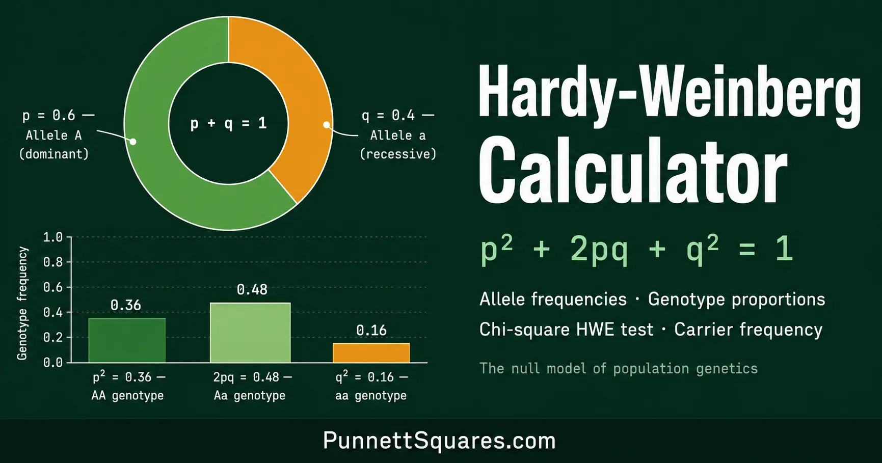
The Hardy-Weinberg principle establishes the baseline expectation for a non-evolving population. It states that for a diploid locus with two alleles A (frequency p) and a (frequency q), where p + q = 1, the expected genotype frequencies after a single generation of random mating are p², 2pq, and q² — and these frequencies will remain constant in every subsequent generation, provided the five equilibrium conditions hold.

The Hardy-Weinberg Equation

p² + 2pq + q² = 1

p²

AA genotype

Homozygous dominant

2pq

Aa genotype

Heterozygous carrier

q²

aa genotype

Homozygous recessive

Also: p + q = 1 (allele frequencies must sum to 1)

The equation is derived from the binomial expansion of (p + q)² = p² + 2pq + q². It reflects the fact that, during random mating, each parent independently passes one of their two alleles to the offspring. The probability of AA is p × p = p²; of Aa is (p × q) + (q × p) = 2pq; of aa is q × q = q². For further mathematical derivation, the NCBI Human Molecular Genetics chapter on population genetics provides a rigorous treatment.

Five Conditions for Hardy-Weinberg Equilibrium

HWE only holds when all five of the following idealised conditions are met simultaneously. In practice, no real population perfectly satisfies all five — but large, randomly mating populations often approximate HWE at most loci, making it a useful practical baseline.

No mutation

New mutations at the locus of interest do not arise, and existing alleles are not converted to other alleles during DNA replication. In practice, mutation rates at individual loci are so low (~10⁻⁸ per generation) that this condition is approximately met at most human loci on generational timescales.

Random mating (panmixia)

All individuals in the population mate randomly without any preference for or against specific genotypes. Non-random mating includes inbreeding (preferential mating between relatives), assortative mating (preference for similar phenotypes), and disassortative mating — all of which alter heterozygosity without changing allele frequencies.

No gene flow

No individuals migrate into or out of the population carrying different allele frequencies. Immigration of individuals from a genetically distinct population introduces new alleles and can rapidly shift allele and genotype frequencies away from HWE expectations.

Infinite (large) population size

In finite populations, allele frequencies drift randomly from generation to generation by chance — a process called genetic drift. Drift is strongest in small populations (effective population size Ne < 100) and can cause significant HWE deviation even without any selection or other forces.

No natural selection

All three genotypes (AA, Aa, aa) must have identical fitness — equal probability of surviving to reproductive age and equal reproductive success. Any fitness difference between genotypes (selective advantage or disadvantage) will alter genotype frequencies and eventually shift allele frequencies away from equilibrium.

Real-World Applications of Hardy-Weinberg in Genetics

Medical genetics — estimating carrier frequency for recessive diseases

HWE allows clinicians to estimate the frequency of heterozygous carriers for autosomal recessive conditions from disease prevalence data alone. If the frequency of affected individuals (q²) is known, then q = √(q²), p = 1 − q, and the carrier frequency = 2pq.

Example: Cystic Fibrosis in European populations

Disease frequency (q²): 1/2500 = 0.0004

Recessive allele frequency (q): √0.0004 = 0.02

Dominant allele frequency (p): 1 − 0.02 = 0.98

Carrier frequency (2pq): 2 × 0.98 × 0.02 ≈ 0.039 ≈ 1 in 25

GWAS quality control — detecting genotyping errors

In genome-wide association studies (GWAS), Hardy-Weinberg testing is a standard quality control step. Control samples should be in HWE at the vast majority of loci. Systematic HWE deviation in control samples at a specific SNP typically indicates a genotyping error — cluster plot misalignment, batch effects, or platform-specific artefacts — rather than a genuine biological signal. Loci with HWE p-values below 10⁻⁶ in controls are typically excluded from analysis.

Forensic genetics — DNA profile interpretation

Forensic DNA databases assume HWE when calculating the probability of a random match between a crime scene profile and an unrelated individual. The probability of a specific heterozygous genotype at a locus is estimated as 2p₁p₂ (where p₁ and p₂ are the frequencies of the two alleles) under HWE. Deviations from HWE in the relevant population database can affect the accuracy of match probability calculations used in court.

Conservation biology — detecting inbreeding in threatened species

Small or fragmented populations of endangered species often show HWE deviation — specifically, a deficit of heterozygotes relative to HWE predictions. This heterozygosity deficit is a key indicator of inbreeding depression. Conservation geneticists use HWE testing across multiple microsatellite loci to quantify inbreeding coefficients and guide breeding programmes designed to maximise genetic diversity.

Worked Example — HWE Calculation and Chi-Square Test

A geneticist surveys a population of 1000 individuals for the MN blood group system and observes: 360 MM (AA), 480 MN (Aa), and 160 NN (aa) individuals. Is this population in Hardy-Weinberg equilibrium?

Step 1 — Calculate allele frequencies

Total alleles = 2 × 1000 = 2000

p (M allele) = (2 × 360 + 480) ÷ 2000 = 1200 ÷ 2000 = 0.60

q (N allele) = (2 × 160 + 480) ÷ 2000 = 800 ÷ 2000 = 0.40

Check: p + q = 0.60 + 0.40 = 1.00 ✓

Step 2 — Calculate expected genotype counts

Expected MM = p² × N = 0.36 × 1000 = 360

Expected MN = 2pq × N = 0.48 × 1000 = 480

Expected NN = q² × N = 0.16 × 1000 = 160

Step 3 — Chi-square test

χ² = (360−360)²/360 + (480−480)²/480 + (160−160)²/160

χ² = 0 + 0 + 0 = 0.000

χ² (0.000) < critical value (3.841)

✓ Fail to reject H₀ — population IS in Hardy-Weinberg equilibrium

Try this example yourself: enter 360, 480, 160 in the "Observed genotype counts" mode above.

Frequently Asked Questions — Hardy-Weinberg Equilibrium

What is Hardy-Weinberg equilibrium?

Hardy-Weinberg equilibrium (HWE) is the theoretical state of a diploid population in which allele and genotype frequencies remain constant from generation to generation because no evolutionary forces are acting. It was independently described by G.H. Hardy (British mathematician) and Wilhelm Weinberg (German physician) in 1908. HWE provides the null model in population genetics — deviations from it indicate that mutation, selection, genetic drift, gene flow, or non-random mating is occurring.

What is the Hardy-Weinberg equation p² + 2pq + q² = 1?

For a gene with two alleles A (dominant, frequency p) and a (recessive, frequency q), where p + q = 1, the Hardy-Weinberg equation predicts expected genotype frequencies after one generation of random mating: p² = frequency of AA (homozygous dominant), 2pq = frequency of Aa (heterozygous), q² = frequency of aa (homozygous recessive). These three terms sum to 1 (100% of the population). The equation is derived from the binomial expansion of (p + q)².

How do you calculate allele frequency from genotype counts?

Given observed counts of AA, Aa, and aa individuals in a population sample: total alleles = 2 × (AA + Aa + aa); frequency of A allele (p) = (2 × AA + Aa) ÷ total alleles; frequency of a allele (q) = (2 × aa + Aa) ÷ total alleles. Equivalently, q = 1 − p. This method counts alleles directly — each AA individual contributes 2 A alleles, each Aa contributes 1, and each aa contributes 0.

What are the five conditions for Hardy-Weinberg equilibrium?

The five conditions are: (1) No mutation — allele frequencies are not altered by new mutations at the locus. (2) Random mating (panmixia) — all mating combinations occur in proportion to genotype frequencies. (3) No gene flow — no immigration or emigration of individuals carrying different allele frequencies. (4) Infinite (or very large) population size — random genetic drift does not alter allele frequencies. (5) No natural selection — all genotypes survive and reproduce with equal fitness. In reality, no natural population perfectly meets all five conditions, but large randomly mating populations often approximate HWE at most loci.

How do you test for deviation from Hardy-Weinberg equilibrium?

The chi-square goodness-of-fit test is used: χ² = Σ[(observed − expected)² ÷ expected] across the three genotype classes. With 1 degree of freedom (for a biallelic locus), a χ² value greater than 3.841 indicates significant deviation from HWE at the p = 0.05 significance level. The degrees of freedom = number of genotype classes − number of estimated parameters − 1 = 3 − 1 − 1 = 1.

What does deviation from Hardy-Weinberg equilibrium mean?

Significant deviation from HWE indicates that one or more evolutionary forces are acting on the locus — or that there is a problem with the data. Excess homozygosity (observed homozygotes > expected) suggests inbreeding, population stratification, or positive selection. Excess heterozygosity suggests balancing selection or outbreeding. In GWAS quality control, HWE deviation in control samples often signals genotyping errors. In natural populations, deviation may reflect local adaptation, recent bottlenecks, or migration.

How is Hardy-Weinberg equilibrium used in medical genetics?

HWE is routinely used to estimate carrier frequencies for autosomal recessive diseases. If the disease frequency (q²) is known from epidemiology, then q = √(q²), and the carrier frequency = 2pq. For cystic fibrosis in Europeans (disease frequency ≈ 1/2500), q = √(1/2500) = 0.02, giving a carrier frequency of 2 × 0.98 × 0.02 ≈ 1/25. This assumes the population is in HWE at the CFTR locus — reasonable for large outbred populations.

What is the carrier frequency formula in Hardy-Weinberg genetics?

Under HWE, the carrier (heterozygous) frequency is 2pq. Since p = 1 − q, the formula can be written as 2q(1 − q). For rare recessive conditions where q is small, p ≈ 1 and the carrier frequency ≈ 2q. This means carriers are approximately 2/q times more frequent than affected individuals (q²). For q = 0.02 (cystic fibrosis), carriers are 2/0.02 = 100 times more common than affected individuals.