How to Calculate Fst: Formula and Worked Example

Calculating Fst comes down to one comparison: how much genetic diversity sits inside your subpopulations versus how much sits in the whole sample pooled together. The smaller the diversity within groups relative to the diversity in the total, the more those groups have diverged, and the higher the Fst. Every estimator you will meet, from Wright's original formula to the modern ones built into sequencing software, is a different way of making that one simple comparison rigorous and unbiased.

This guide walks through an actual calculation by hand using Nei's heterozygosity method, which is the most transparent way to see what the number is doing. Then it explains why the estimator that most software actually uses, Weir and Cockerham's, looks more complicated, and when you should reach for it instead. If you want the conceptual background first, our explainer on what Fst is covers the underlying idea before the arithmetic.

The Formula You Can Do by Hand

Masatoshi Nei gave Fst its most teachable form in 1973. It is built from heterozygosity, the probability that two randomly chosen alleles at a locus are different. You need two versions of it.

The first is HS, the average expected heterozygosity within your subpopulations. You calculate the expected heterozygosity inside each subpopulation from that subpopulation's own allele frequencies, then average across subpopulations. The second is HT, the expected heterozygosity of the total population, which you get by first averaging the allele frequencies across all subpopulations and then computing heterozygosity from those pooled frequencies.

With both in hand, the formula is short:

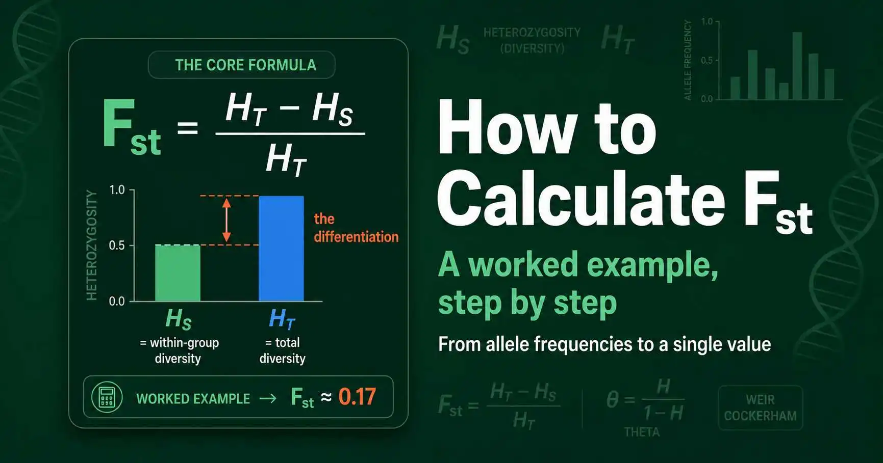
Fst = (HT − HS) / HT

The logic is worth restating because it makes the whole calculation intuitive. HT is the diversity you would expect if everyone bred as one pool. HS is the diversity that actually exists within groups. When subdivision has caused groups to differ, each group individually holds less diversity than the whole, so HS comes in below HT, and the proportional gap between them is Fst. The steps below put numbers to that.

Worked Example: Three Steps

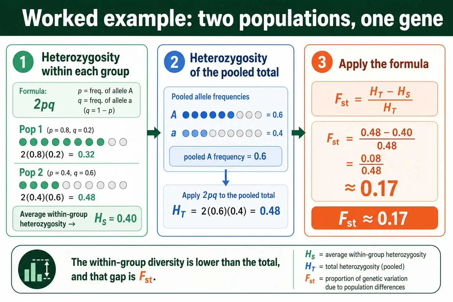
Take a single gene with two alleles, A and a, sampled in two subpopulations. In subpopulation 1, the frequency of A is 0.8. In subpopulation 2, the frequency of A is 0.4. We will find Fst in three steps.

Step 1: Heterozygosity within each subpopulation

Expected heterozygosity for a two-allele locus is 2pq, where p and q are the two allele frequencies. For subpopulation 1, p is 0.8 and q is 0.2, so the heterozygosity is 2 times 0.8 times 0.2, which is 0.32. For subpopulation 2, p is 0.4 and q is 0.6, so the heterozygosity is 2 times 0.4 times 0.6, which is 0.48.

Average these to get HS. The mean of 0.32 and 0.48 is 0.40. So HS, the average within-subpopulation heterozygosity, is 0.40.

Step 2: Heterozygosity of the total population

First average the allele frequencies across the two subpopulations. The frequency of A is the mean of 0.8 and 0.4, which is 0.6, so the frequency of a is 0.4. Now compute heterozygosity from these pooled frequencies: HT is 2 times 0.6 times 0.4, which is 0.48.

Notice that HT, at 0.48, is larger than HS, at 0.40. That gap is the whole story. Pooling the populations creates more apparent diversity than exists within either group, precisely because the groups have different allele frequencies.

Step 3: Apply the formula

Fst = (HT − HS) / HT = (0.48 − 0.40) / 0.48 = 0.08 / 0.48 ≈ 0.167

So Fst is about 0.17. By Wright's rough guideposts that signals great differentiation, which fits a gene whose frequency swings from 0.8 in one group to 0.4 in the other. The arithmetic never gets harder than this; real datasets just repeat it across many loci and average the results.

Doing It With More Than Two Alleles

Most real markers have more than two alleles, but the method barely changes. The only difference is how you compute heterozygosity. For a locus with any number of alleles, expected heterozygosity is 1 minus the sum of the squared allele frequencies. This single formula reduces to 2pq when there are exactly two alleles, so it is the general version of the same idea. The more alleles a locus carries, the higher its baseline heterozygosity, which is part of why marker choice influences the Fst you can observe.

Suppose a locus has three alleles at frequencies 0.5, 0.3, and 0.2 in a subpopulation. The squared frequencies are 0.25, 0.09, and 0.04, summing to 0.38, so the heterozygosity is 1 minus 0.38, which is 0.62. You would do this for each subpopulation to build HS, average the allele frequencies across subpopulations to get the pooled frequencies, compute HT from those, and apply the same (HT − HS) / HT formula. Nothing about the structure of the calculation changes; only the heterozygosity formula generalizes.

Across multiple loci, the standard practice is to compute the components and combine them carefully rather than simply averaging the per-locus Fst values. As work by Gaurav Bhatia, Nick Patterson, and colleagues showed in a 2013 paper in Genome Research, averaging the numerator and denominator separately across loci, a "ratio of averages," behaves better than averaging the individual Fst values, an "average of ratios." That subtle choice was enough to explain a real discrepancy between published Fst estimates from the HapMap and 1000 Genomes projects.

Why Software Uses a Different Formula

If you run Fst in a program like VCFtools or the scikit-allel library, you will not get Nei's formula. You will almost always get the estimator that Bruce Weir and C. Clark Cockerham published in Evolution in 1984, and it looks far more involved. There is a good reason for the extra machinery.

Nei's formula, applied directly to a sample, is biased. When you sample a limited number of individuals, the random noise of sampling makes subpopulations look more different than they truly are, which inflates Fst, and the bias is worst for small samples. Weir and Cockerham reframed the whole problem in the language of analysis of variance, the same statistical framework used to partition variation in experiments. They split the total genetic variation into components: variation among populations, among individuals within populations, and within individuals. Writing those three variance components as a, b, and c, their estimator of Fst, which they called θ, is simply a divided by the sum of a, b, and c.

The payoff is that θ corrects for finite and unequal sample sizes, so it returns an unbiased estimate where Nei's direct formula would not. Their approach built on an earlier coancestry-based distance measure from a 1983 paper by John Reynolds, Weir, and Cockerham in the journal Genetics.

To see why the correction matters, picture sampling just five individuals from each of two genuinely identical populations. By bad luck, the five you draw from one population might carry slightly different allele frequencies than the five from the other, purely from the small sample. Nei's uncorrected formula would read that accidental difference as real differentiation and report a positive Fst, even though the true value is zero. Weir and Cockerham's estimator explicitly accounts for the sampling variance, subtracting out the portion of the apparent difference that the sample size alone can explain, so it correctly returns a value near zero. The smaller and more uneven the samples, the larger this correction becomes, which is exactly why it is indispensable for the modest sample sizes common in wildlife and conservation studies.

For anyone reporting Fst from real samples, θ is the responsible default, which is why it is baked into the standard tools. You rarely compute it by hand, but it answers the exact same question Nei's formula does, just with the sampling noise stripped out.

A Note on Other Estimators

Weir and Cockerham's θ is the workhorse, but it is not the only modern estimator, and the differences matter when precision counts.

The Hudson estimator, drawn from a 1992 paper by Richard Hudson, Montgomery Slatkin, and Wayne Maddison, computes Fst from the difference between within-population and between-population diversity in a way that is independent of sample size. In their 2013 analysis, Bhatia and colleagues recommended the Hudson estimator specifically because it does not depend on how many populations you sample or how evenly, a property that becomes important in large human genetic studies. For pairwise comparisons between two populations especially, the Hudson and Weir-Cockerham estimators tend to agree closely when sample sizes are similar.

The choice among estimators usually changes Fst only modestly, but the changes are not random. Nei's Gst tends to read higher than the others, while the sample-size corrections in θ and the Hudson estimator tend to pull values down toward the truth. The practical advice from the methodological literature is consistent: pick a sample-size-corrected estimator, state which one you used, and apply it consistently, because comparing an Fst computed one way against an Fst computed another way can mislead.

Pairwise Versus Global Fst

When you have more than two subpopulations, you face a choice that trips up newcomers: do you calculate one overall Fst, or a separate value for every pair? Both are legitimate, and they answer different questions.

A global Fst summarizes differentiation across all your subpopulations at once, giving a single number for how structured the whole sample is. It is the right choice when you want one headline figure for a species or region. A pairwise Fst, by contrast, is computed separately for each pair of subpopulations, producing a matrix of values. That matrix is far more informative when populations differ in how related they are, because it reveals which specific pairs are similar and which are divergent.

Pairwise matrices are what let researchers see structure rather than just measure it. Two populations that exchange migrants might show a pairwise Fst near zero, while a third, isolated population shows high Fst against both. A global value would blur all of that into one average, hiding the pattern. In practice, studies often report both: a global Fst to set the overall scale, and a pairwise matrix to map the relationships. Weir and Cockerham's framework handles both, with the pairwise case simply setting the number of populations to two for each comparison.

Testing Whether Fst Is Significant

A raw Fst value, on its own, does not tell you whether the differentiation is statistically real or could have arisen by sampling chance. For that, you need a measure of uncertainty, and careful analyses always pair an Fst estimate with one.

The usual approach is resampling. By bootstrapping over loci, repeatedly recalculating Fst from random subsets of the genetic markers with replacement, software builds a confidence interval around the estimate. If that interval excludes zero, the differentiation is unlikely to be a fluke. A related technique, jackknifing over loci, was recommended by Weir and Cockerham themselves as a way to attach a variance to an Fst estimate, and it remains common. In permutation tests, individuals are shuffled randomly among populations many times to build a null distribution of Fst values expected under no structure, against which the observed value is compared.

This step matters most when Fst is small. A value of 0.01 might be real, reflecting weak but genuine structure in a large, well-sampled dataset, or it might be indistinguishable from zero in a small one. Without a confidence interval, you cannot tell the two situations apart. The number alone is never the whole answer; its uncertainty is part of the result, and reporting an Fst without it leaves the most important interpretive question open.

Starting From Genotype Counts

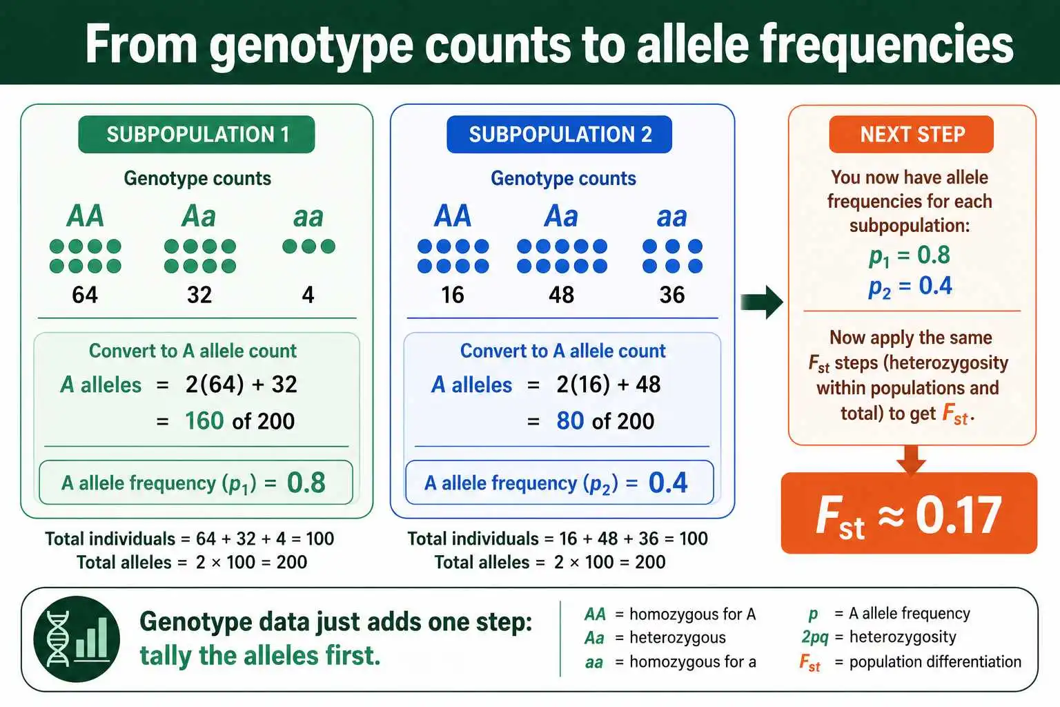
Often you do not begin with allele frequencies at all; you begin with counts of genotypes, and have to derive the frequencies first. Working an example from that starting point shows the full pipeline.

Imagine genotyping 100 individuals in each of two subpopulations at a single two-allele locus. In subpopulation 1, you count 64 AA, 32 Aa, and 4 aa. In subpopulation 2, you count 16 AA, 48 Aa, and 36 aa. To get the frequency of allele A in subpopulation 1, count the A alleles: each AA contributes two and each Aa contributes one, so that is 2 times 64 plus 32, which is 160, out of 200 total alleles, giving a frequency of 0.8. In subpopulation 2, the A alleles number 2 times 16 plus 48, which is 80, out of 200, giving 0.4.

Those are the same 0.8 and 0.4 frequencies from the first worked example, so the rest follows identically: HS works out to 0.40, HT to 0.48, and Fst to about 0.17. The lesson is that genotype data simply adds one preliminary step, converting counts to frequencies by tallying alleles, before the heterozygosity calculation begins. Real software does exactly this internally, reading genotypes and producing allele frequencies before any Fst formula is applied.

One subtlety is worth flagging. The observed genotype counts also let you check whether each subpopulation is in Hardy-Weinberg proportions, which the standard Fst calculation quietly assumes when it computes expected heterozygosity from allele frequencies. If a subpopulation is itself inbred or internally structured, its observed heterozygosity will fall below the expected 2pq, which is the territory of Fis rather than Fst. Separating these is exactly what Weir and Cockerham's three-component framework was designed to do, partitioning variation among populations, among individuals within populations, and within individuals at once.

Common Pitfalls

A handful of mistakes account for most wrong Fst values, and they are easy to sidestep once you know them.

The first is averaging per-locus Fst values directly across loci, instead of combining the variance components and taking a ratio of averages. The second is forgetting that highly polymorphic markers, like microsatellites, cap the maximum possible Fst well below 1, so a "low" value from such a marker can still represent strong differentiation. The third is using Nei's uncorrected formula on small samples and reading the inflated result as real differentiation rather than sampling noise. And the fourth is comparing Fst values calculated with different estimators or different marker types as if they were interchangeable, when they are not strictly comparable.

None of these are hard to avoid. They mostly come down to using a sample-size-corrected estimator, knowing your marker's properties, and being consistent. A final habit worth adopting is to always report the number of loci and individuals behind an Fst value, since the same number carries very different weight when it rests on ten markers versus ten thousand. With those practices in place, the calculation is reliable, and the worked example above scales straight up to genome-wide data.

The Tools That Compute It

In real research, almost nobody computes genome-wide Fst by hand. A set of well-established software tools does the work, and knowing what they implement helps you read the methods section of any population genetics paper.

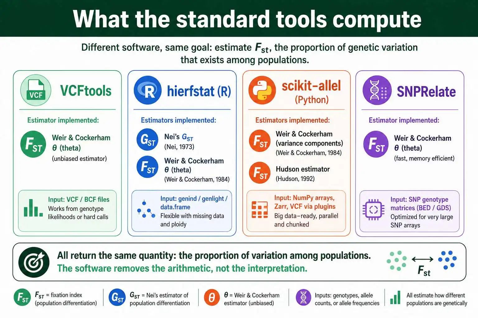
VCFtools, a long-standing command-line program, computes Weir and Cockerham's θ directly from variant call files and is probably the most cited Fst tool in the genomics literature. The R package hierfstat implements both Nei's and Weir and Cockerham's estimators and is popular for smaller datasets and teaching, while the Python library scikit-allel provides fast, scriptable Fst functions, including the Weir and Cockerham variance components and the Hudson estimator, built for genome-scale data. For SNP array data, packages like SNPRelate handle very large samples efficiently.

What unites these tools is that they all return the same kind of quantity, the proportion of variation among populations, and they all face the same choices this guide has covered: which estimator, how to combine across loci, and how to attach confidence intervals. The software removes the arithmetic, not the interpretation. A value of Fst still has to be read against the biology of the organism and the markers used, which is why understanding the calculation by hand pays off even when a program does it for you. Where these numbers come from biologically, the balance of genetic differentiation and gene flow, is what gives any computed value its meaning.

Frequently Asked Questions

What is the simplest way to calculate Fst by hand?

Use Nei's heterozygosity method. Find the average expected heterozygosity within your subpopulations (HS), find the expected heterozygosity of the pooled total population (HT), then compute Fst as (HT − HS) divided by HT. For a two-allele locus, expected heterozygosity is just 2pq.

Why does software give a different Fst than my hand calculation?

Because most software uses Weir and Cockerham's θ estimator, which corrects for sampling bias, while a simple hand calculation often uses Nei's uncorrected formula. The corrected estimator returns slightly different, less biased values, especially with small or unequal sample sizes.

Which Fst estimator should I use?

For most purposes, use a sample-size-corrected estimator: Weir and Cockerham's θ is the standard default, and the Hudson estimator is favored in large human genetic studies for being independent of sample size. Whatever you choose, report it and apply it consistently across your comparisons.

From Formula to Real Data

The mechanics of Fst are simpler than its reputation suggests. Compute the diversity within your groups, compute the diversity in the pooled whole, and report the shortfall as a proportion. Nei's formula does this transparently enough to work by hand, and the worked example above, from 0.8 and 0.4 down to an Fst of 0.17, is the entire idea in miniature. Everything the heavy-duty estimators add, the variance-component framework of Weir and Cockerham, the sample-size independence of Hudson, is in service of getting that same proportion right when real sampling noise gets in the way.

When you move to your own data, the one habit worth keeping is consistency: choose a corrected estimator, name it, and use it throughout. To run the calculation on real allele frequencies without doing the arithmetic yourself, try the Fst population differentiation calculator, and to make sense of whatever value you get, our guide on interpreting Fst values explains what counts as high or low.