D coefficient
D = fAB − pA × pB
D equals zero when allele A and allele B associate randomly.
Calculate linkage disequilibrium from AB, Ab, aB, and ab haplotype data. The tool reports allele frequencies, expected haplotypes, D, D′, r², and a practical marker-tagging interpretation.
Use Basic mode for a quick four-count table. Switch to Advanced mode when you have published haplotype frequencies or need a CSV report for a lab worksheet.
Basic mode uses four haplotype counts. Advanced mode adds frequency input and export tools.
Presets help you compare strong LD, weak LD, rare alleles, and negative association.
Use phased haplotype counts when you have them. Use frequency mode when a paper reports frequencies instead of counts.
Live LD result
The loci show LD, but marker tagging remains incomplete.
D
0.175
D′
0.7143
r²
0.4902
pA
0.5
pa
0.5
pB
0.49
pb
0.51
AB
Count 420
Observed 42% · Expected 24.5% · Difference 0.175
Ab
Count 80
Observed 8% · Expected 25.5% · Difference -0.175
aB
Count 70
Observed 7% · Expected 24.5% · Difference -0.175
ab
Count 430
Observed 43% · Expected 25.5% · Difference 0.175
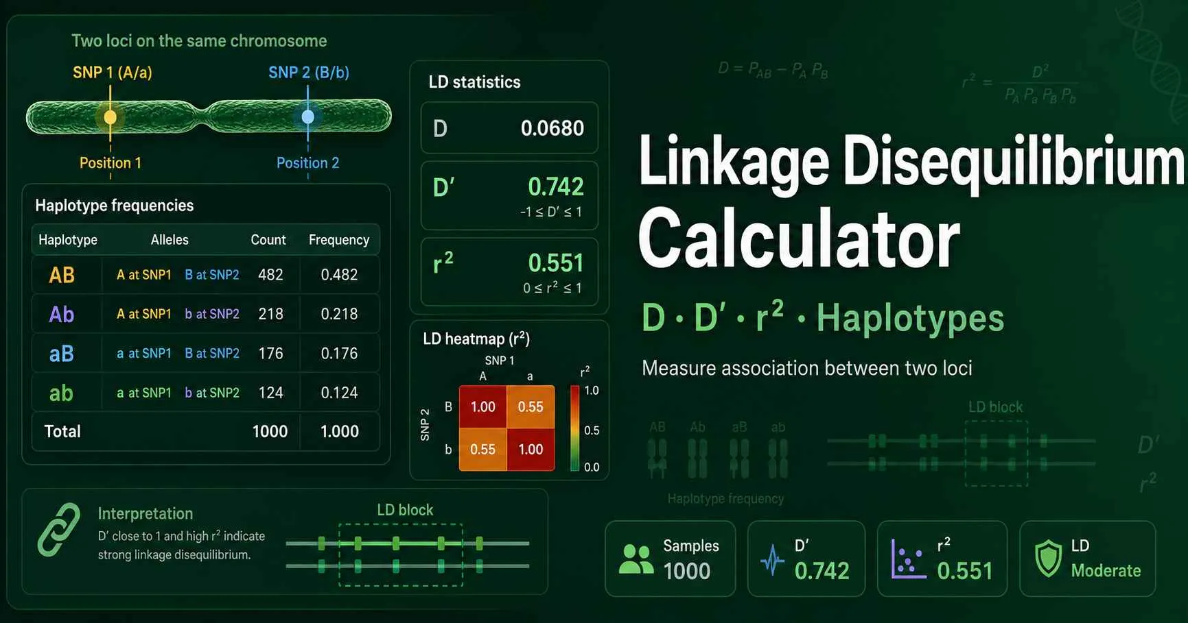
LD answers this question: do two alleles travel together more often than allele frequencies predict? Enter AB, Ab, aB, and ab haplotypes, and the calculator compares observed frequencies with linkage equilibrium expectations.
D measures the raw difference between observed AB and expected AB. D′ rescales D by the maximum possible value under the observed allele frequencies. r² estimates marker correlation, so it helps researchers choose tag SNPs and interpret genome-wide association results.
This page works best after you calculate single-locus allele frequencies. It also complements genetic linkage, because recombination can erode LD across generations.
Each component targets a different part of a two-locus LD calculation. Use the table as a fast reference while you enter data.
Observed two-locus haplotypes
Use phased chromosome counts or direct haplotype observations.
Allele frequencies
Check whether rare alleles limit D′ or r² interpretation.
Raw disequilibrium coefficient
Shows whether AB appears above or below the random expectation.
Scaled disequilibrium
Compares D with its allele-frequency limit.
Marker correlation
Shows how well one marker predicts the other.
D = fAB − pA × pB
D equals zero when allele A and allele B associate randomly.
D′ = D / Dmax
D′ rescales D, so rare allele frequencies can still produce high values.
r² = D² / (pA × pa × pB × pb)
r² gives the clearest tag-marker interpretation for association work.
A data set contains AB = 420, Ab = 80, aB = 70, and ab = 430 haplotypes. The AB and ab classes dominate the table. The calculator returns positive D and a high r² value.
This pattern means allele A often appears with allele B. A researcher could use one marker as a proxy for the other if r² remains high in the study population.
A rare allele can push D′ upward even when r² stays modest. The historical association may look strong, but the marker predicts few chromosomes because one allele appears in only a small fraction of samples.
Use r² when you select tag SNPs. Use D′ when you discuss recombination history, founder haplotypes, or haplotype-block boundaries.
Start with r² when your question involves prediction. A high r² value means one locus captures much of the allele information at the second locus. Genome-wide association tools such as PLINK report haplotype-based LD statistics, including r² and D′, for exactly this kind of marker-pair inspection.
Read D′ as a scaled disequilibrium value. D′ can show strong historical association, but allele frequency can constrain its interpretation. Mathematical reviews of LD statistics emphasize that r² depends strongly on allele frequencies, so rare alleles need careful interpretation.
Add heterozygosity when you compare populations. Population structure, drift, selection, and admixture can all create LD even when two loci sit far apart on a chromosome.
Haplotype LD needs haplotypes. Unphased genotypes require estimation before you calculate D, D′, and r².
Small samples produce unstable haplotype frequencies. Treat low-count classes as warning signs.
Admixed or pooled populations can inflate LD. Interpret pairwise statistics with the sampling design.
Linkage disequilibrium measures whether alleles at two loci occur together more or less often than random association predicts. The calculator compares the observed AB haplotype frequency with the expected frequency pA × pB. A nonzero D value shows allele association. r² then describes how well one marker predicts the other marker in the sample.
Use both, but answer different questions with them. D′ scales D to its maximum possible value, so it often captures historical recombination patterns. r² measures correlation between loci and gives better marker-tagging information for association studies. A pair can show high D′ but low r² when one allele remains rare.
Enter the four two-locus haplotype classes: AB, Ab, aB, and ab. These counts usually come from phased genotype data, family data, microbial sequencing, pooled haplotype calls, or direct chromosome-level observations. Do not enter genotype counts unless you have already converted them into haplotypes. Unphased diploid genotypes need an estimation method before haplotype LD calculation.
Many genetic association workflows treat r² above 0.8 as strong marker tagging. Values between 0.5 and 0.8 often show useful association, while values below 0.2 usually indicate weak tagging. These boundaries work as practical guideposts, not universal biological laws. Study design, allele frequency, recombination, and population history all affect LD interpretation.
D′ can reach 1 when the observed D value hits its allele-frequency limit. r² also depends on allele frequencies at both loci, so rare alleles can keep r² low even when D′ looks complete. This pattern appears often around uncommon variants. For marker selection, r² usually tells you more about predictive value.
No. LD shows statistical allele association in a sample, not direct proof of physical closeness. Physical linkage, selection, admixture, founder effects, drift, and population structure can all create LD. You need map position, recombination data, or sequence context to interpret the biological cause. Use this page as a first analysis step before deeper population-genetic modeling.
Recombination breaks down associations between alleles over generations. Closely spaced loci often retain LD longer because crossovers rarely separate them. Distant loci can still show LD after bottlenecks, admixture, selection, or recent mutation. That is why LD analysis works best when you interpret r² and D′ alongside genomic distance and population history.