How to Use the Hardy-Weinberg Equation (Steps)

To use the Hardy-Weinberg equation, you almost always start with q², the frequency of the homozygous recessive genotype, because it is the only genotype you can identify directly from the phenotype. Take its square root to find q, the recessive allele frequency. Then use p + q = 1 to find p. Square p to get p², the homozygous dominant frequency, and calculate 2pq for the heterozygous frequency. Finally, check that p² + 2pq + q² adds up to 1. That sequence solves the vast majority of Hardy-Weinberg problems.

The equation looks intimidating with its squares and cross terms, but it follows a fixed, repeatable procedure once you know the order of steps. This guide walks through that procedure step by step, works several complete examples, and covers the one variation where you start from the dominant phenotype instead. Learn the sequence and these problems become routine. The calculation can be checked with a calculator, but working through the steps by hand is what builds real understanding.

The Two Equations You Are Working With

Before the steps, it helps to have both Hardy-Weinberg equations clearly in view, since every problem uses them together. The first handles allele frequencies and the second handles genotype frequencies, and the whole procedure is just moving between them.

The first equation is p + q = 1. Here p is the frequency of the dominant allele and q is the frequency of the recessive allele, and they sum to 1 because together they make up all the copies of the gene. The second equation is p² + 2pq + q² = 1. This one gives the genotype frequencies: p² is the proportion of homozygous dominant individuals, 2pq is the proportion of heterozygotes, and q² is the proportion of homozygous recessive individuals. These three also sum to 1 because they account for everyone in the population.

The reason you can move so freely between these equations is that they share the same p and q. Once you know the allele frequencies, you can find any genotype frequency, and once you know certain genotype frequencies, you can find the allele frequencies. The art of solving a problem is choosing the right entry point, then following the chain. For the conceptual background on what these equations mean, our guide on what Hardy-Weinberg equilibrium is explains the principle behind the math.

Why You Start With q²

The single most important habit in Hardy-Weinberg problems is to start with q², and understanding why makes every problem easier. The reason comes down to which genotype you can actually identify by looking at a population.

With complete dominance, the homozygous dominant individuals (genotype AA) and the heterozygotes (genotype Aa) look exactly the same, because the dominant allele masks the recessive one in both. You cannot tell them apart by phenotype, so you cannot directly count either group on its own. The homozygous recessive individuals (genotype aa) are different. They are the only ones showing the recessive phenotype, so their frequency is something you can observe and count directly. That observable frequency is q².

This is why nearly every Hardy-Weinberg problem hands you information about the recessive phenotype. It is the only phenotype that maps to a single genotype, making it the natural starting point. From q² you can reach everything else: the square root gives q, then p + q = 1 gives p, and from p and q you can find p² and 2pq. The recessive phenotype is the key that unlocks the whole population. The mnemonic worth memorizing is simple: start with q², then take the square root. Lock that in and you will rarely get stuck.

It is worth appreciating just how much information the recessive phenotype carries. From that one observable proportion, you derive both allele frequencies and all three genotype frequencies, a complete description of the gene across the entire population. This is remarkable because allele frequencies are otherwise hard to measure directly, you cannot look at a person and read off whether a dominant individual is homozygous or heterozygous. The recessive phenotype sidesteps that problem entirely, because it corresponds to exactly one genotype. In real research and medicine, the frequency of a recessive condition is often known from health records, which is precisely why the q² starting point is not just a classroom convenience but the standard way these calculations are done in practice.

The Step-by-Step Procedure

Here is the full procedure that solves a standard Hardy-Weinberg problem, laid out as a sequence you can follow every time. Each step builds on the previous one, moving from the one thing you can observe to the complete genetic picture.

Step one: identify q². Find the frequency of the homozygous recessive individuals, which is the proportion showing the recessive phenotype, and set that equal to q². Step two: solve for q by taking the square root of q². Step three: solve for p using p + q = 1, so p equals 1 minus q. Step four: find p² by squaring p, giving the homozygous dominant frequency. Step five: find 2pq by multiplying 2 times p times q, giving the heterozygous frequency.

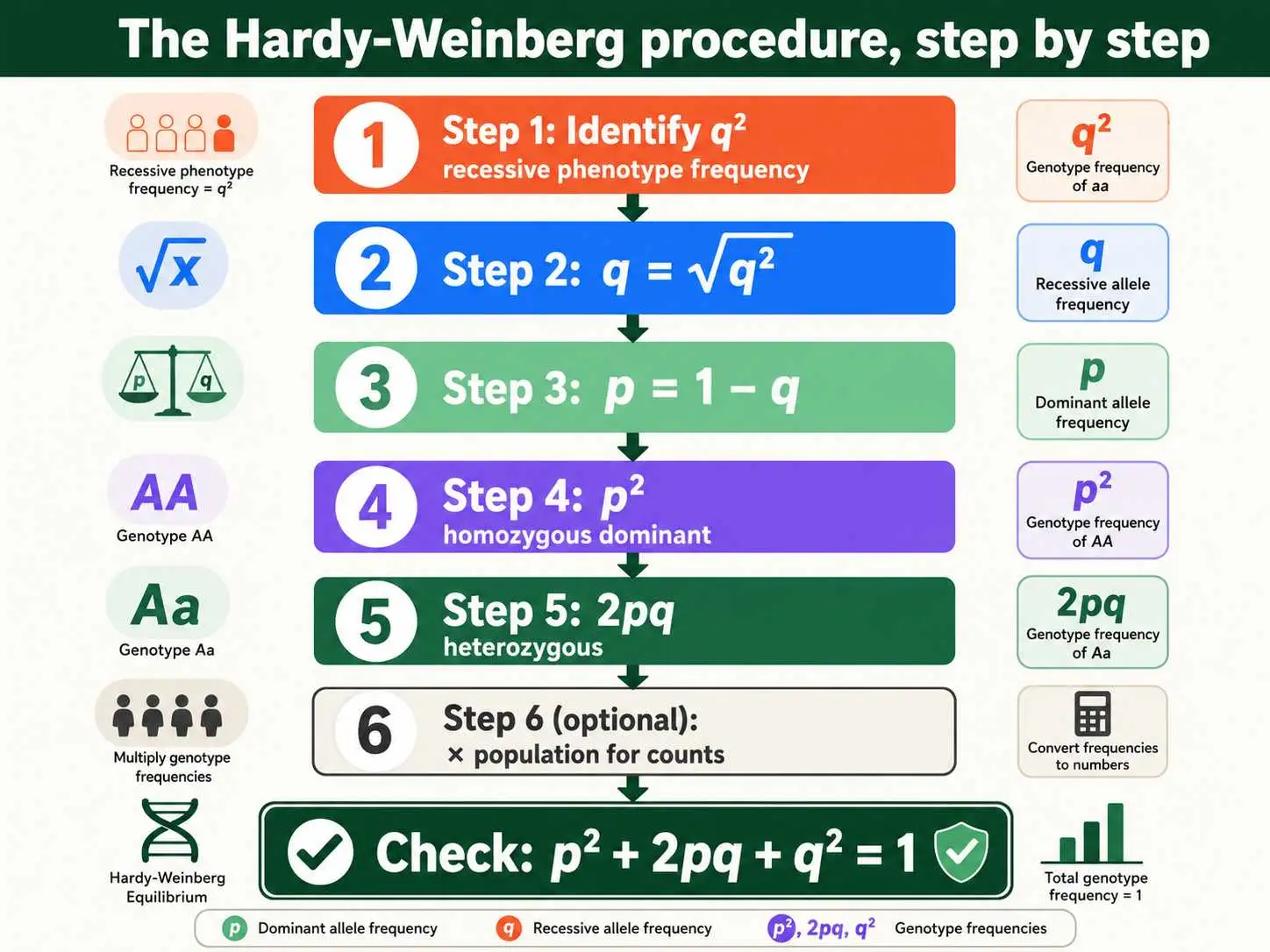
There is an optional sixth step when a problem asks for actual numbers of individuals rather than frequencies. To get counts, multiply each genotype frequency by the total population size. So the number of homozygous dominant individuals is p² times the total, the number of heterozygotes is 2pq times the total, and the number of homozygous recessive individuals is q² times the total. Whatever the problem asks for, finish by verifying that p² + 2pq + q² equals 1, which confirms your arithmetic. This verification step catches almost any calculation error before you commit to an answer, and it takes only a moment, so it is always worth doing even when you are confident the arithmetic is right.

Worked Example 1: Starting From the Recessive Phenotype

Take a concrete problem. In a population of 1,000 individuals, 90 show a recessive trait. Find the allele frequencies and all the genotype frequencies. This is the most common form of Hardy-Weinberg question.

Start with q². The 90 individuals showing the recessive trait are homozygous recessive, so q² equals 90 divided by 1,000, which is 0.09. Take the square root to find q, which is the square root of 0.09, giving 0.3. Now use p + q = 1, so p equals 1 minus 0.3, which is 0.7. You now have both allele frequencies: the dominant allele A is at 0.7 and the recessive allele a is at 0.3.

Now find the remaining genotype frequencies. The homozygous dominant frequency p² is 0.7 squared, which is 0.49, so 49 percent of the population is AA. The heterozygous frequency 2pq is 2 times 0.7 times 0.3, which is 0.42, so 42 percent is Aa. You already know q² is 0.09, so 9 percent is aa. Check the sum: 0.49 plus 0.42 plus 0.09 equals 1, confirming the answer.

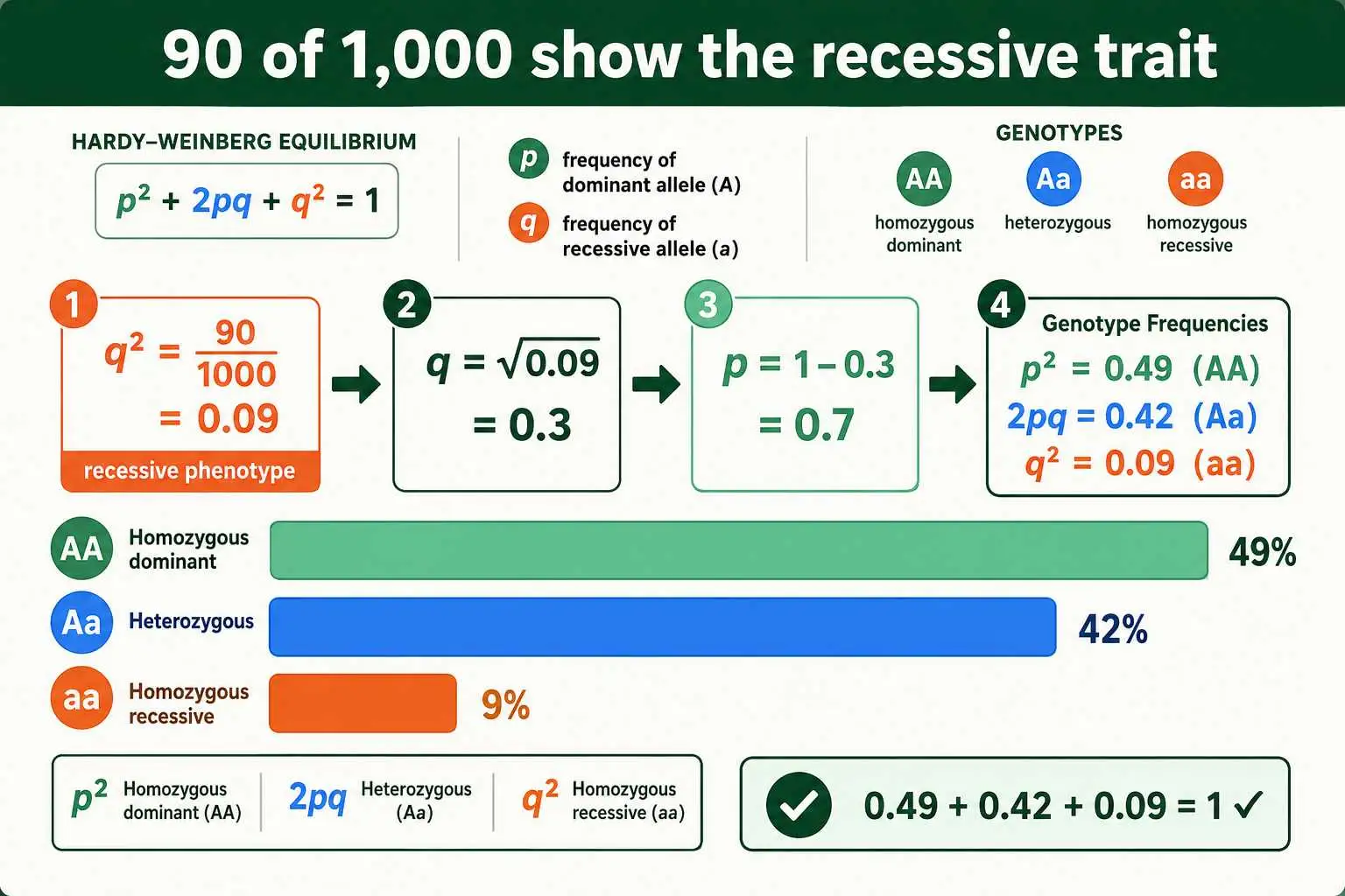
If the problem wanted counts, you would multiply by 1,000 to get 490 AA, 420 Aa, and 90 aa individuals. From a single observed number, the 90 affected individuals, you have reconstructed the entire genetic structure of the population.

Worked Example 2: Finding the Carrier Frequency

A very common variation asks specifically for the carrier frequency, the proportion of heterozygotes, which is often the most useful number in real applications. The procedure is the same, you just report the 2pq value.

Suppose a recessive condition affects 1 in 10,000 people, and you want to know what fraction of the population carries the allele without being affected. Start with q². The affected frequency is 1 in 10,000, so q² equals 0.0001. The square root gives q equals 0.01. Then p equals 1 minus 0.01, which is 0.99. The carrier frequency is 2pq, which is 2 times 0.99 times 0.01, giving 0.0198, or about 2 percent.

The result is revealing. While only 1 in 10,000 people is affected, roughly 1 in 50 is a carrier, which is two hundred times more common. This large gap between carriers and affected individuals is a general feature of rare recessive alleles, and it has real importance in genetics counseling and public health. The carrier calculation is so commonly needed that we devote a full guide to calculating carrier frequency, but the core of it is simply the 2pq step of the standard procedure. The same logic underlies real genetic screening programs, which use the known frequency of a condition to estimate how many people in a population unknowingly carry the allele.

Worked Example 3: Calculating Numbers of Individuals

Some problems ask not for frequencies but for the actual number of individuals of each genotype, which uses the optional sixth step. Once you have the frequencies, you simply scale them up by the population size.

Imagine a population of 1,000 cats where coat color follows a single gene, and 360 cats show the dominant black coat from genotype BB, but you are told the recessive allele frequency q is 0.4 and asked how many cats of each genotype there are. First find the frequencies. With q equal to 0.4, p equals 0.6. So p² is 0.36, 2pq is 2 times 0.6 times 0.4 which is 0.48, and q² is 0.16. These frequencies must sum to 1, and 0.36 plus 0.48 plus 0.16 does equal 1.

Now convert to counts by multiplying each frequency by the total population of 1,000. The homozygous dominant count is 0.36 times 1,000, which is 360 cats with genotype BB. The heterozygous count is 0.48 times 1,000, which is 480 cats with genotype Bb. The homozygous recessive count is 0.16 times 1,000, which is 160 cats with genotype bb. Adding these gives 360 plus 480 plus 160, which equals the full 1,000, confirming the work. This counts version of the procedure is common in exam questions and in real population studies, where researchers want concrete numbers rather than proportions. The step is straightforward: solve for frequencies as usual, then multiply each by the total population at the end.

What the Genotype Frequencies Tell You

Beyond the mechanics, it is worth pausing on what the numbers actually mean, because interpreting them is often the real point of a problem. The three genotype frequencies paint a complete picture of how a gene is distributed across a population.

The p² value tells you how common the homozygous dominant genotype is, the individuals carrying two dominant alleles. The q² value tells you how common the affected or homozygous recessive individuals are, which for a disease allele is the proportion of the population that shows the condition. The 2pq value, the heterozygotes, is frequently the most important in practice, because for a recessive condition these are the unaffected carriers who can still pass the allele to their children. A genetic counselor cares enormously about this carrier number.

A recurring and counterintuitive lesson emerges from these values when an allele is rare. When q is small, q² is very small but 2pq is much larger, so carriers vastly outnumber affected individuals. A recessive allele can therefore be quite common in a population while the condition it causes remains rare, because most copies of the allele sit hidden in healthy carriers. This is why recessive alleles persist over generations rather than being eliminated, and it is one of the most important practical insights the Hardy-Weinberg equation provides. Reading the genotype frequencies, rather than just calculating them, is what turns the math into biological understanding.

The Variation: Starting From the Dominant Phenotype

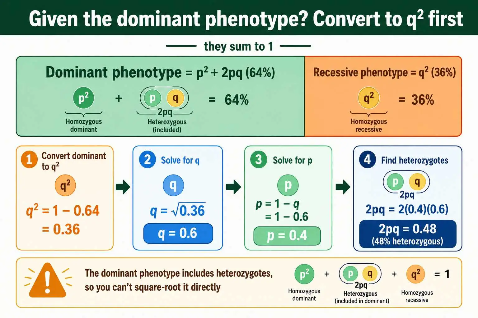
Occasionally a problem gives you the frequency of the dominant phenotype instead of the recessive one, and this requires a small extra step. Because the dominant phenotype includes both the homozygous dominant and heterozygous individuals, it equals p² plus 2pq, which is not a single clean term you can square-root.

The trick is to use the complement. Since all genotype frequencies sum to 1, the frequency of the dominant phenotype plus the frequency of the recessive phenotype must also equal 1. So if you know the dominant phenotype frequency, you subtract it from 1 to find q², the recessive phenotype frequency. From there, the standard procedure takes over: square-root q² to get q, find p, and so on.

For example, suppose 64 percent of a population shows the dominant trait. The recessive phenotype frequency is therefore 1 minus 0.64, which is 0.36, and this equals q². The square root gives q equals 0.6, and p equals 1 minus 0.6, which is 0.4. Now you can find any genotype frequency: 2pq is 2 times 0.4 times 0.6, which is 0.48, so 48 percent are heterozygous. The key insight is to always convert back to q² first, because q² is the only term you can take a clean square root of.

Whatever form the problem takes, routing through q² keeps the procedure consistent.

Common Errors to Avoid

A handful of mistakes account for most wrong answers in Hardy-Weinberg problems, and knowing them keeps you on track. Each one is easy to avoid with a little care.

The most frequent error is setting the recessive phenotype frequency equal to q instead of q². The recessive phenotype frequency is q², the squared term, so you must take its square root to get the allele frequency q. Forgetting the square root, or taking it at the wrong stage, throws off everything downstream. A second common mistake is confusing the dominant phenotype with p². The dominant phenotype includes heterozygotes, so it equals p² plus 2pq, not p² alone. Treating the dominant phenotype as if it were just the homozygous dominant frequency leads to the wrong q².

Another error is forgetting the factor of 2 in the heterozygous term, calculating pq instead of 2pq. Heterozygotes form in two ways, so their frequency is doubled. A final slip is reporting frequencies when the question asked for counts, or vice versa. If a problem gives a population size and asks how many individuals, remember the optional step of multiplying each frequency by the total. Running the sum check at the end, confirming p² + 2pq + q² equals 1, catches most of these errors before they cost you, which is why it is worth doing every time.

When the Equation Applies

A crucial caveat sits behind every Hardy-Weinberg calculation: the genotype frequencies you predict from p and q are only correct if the population is in Hardy-Weinberg equilibrium. The equation does not just describe any population; it describes the specific genotype distribution expected when no evolutionary forces are acting.

This matters most in the predictive direction. When you take allele frequencies and calculate p², 2pq, and q², you are assuming the alleles combine at random, which requires random mating and the absence of selection, drift, migration, and mutation. If the population violates these conditions, the real genotype frequencies can differ from your prediction. For instance, a population with strong inbreeding will have more homozygotes than 2pq predicts, because non-random mating concentrates matching alleles together. The equation would give a technically correct calculation but a biologically wrong prediction for that population.

In practice, this means Hardy-Weinberg predictions are estimates that assume equilibrium, and they are most reliable for large, randomly mating populations without strong selection. The conditions that must hold are spelled out in our guide to the assumptions of Hardy-Weinberg, and they are worth keeping in mind whenever you report a predicted genotype frequency. As the Biology LibreTexts population genetics material emphasises, the equilibrium prediction is a baseline expectation rather than a guaranteed description of reality. The calculation is still useful even when the assumptions are imperfect, because comparing the prediction to the real data is exactly how scientists detect that something evolutionary is happening.

Frequently Asked Questions

What do I start with in a Hardy-Weinberg problem?

Start with q², the frequency of the homozygous recessive individuals, which is the proportion showing the recessive phenotype. It is the only genotype you can identify directly, so it is the entry point. Take its square root to find q, then find p.

How do I find the frequency of heterozygotes?

Calculate 2pq. Once you have the allele frequencies p and q, multiply 2 times p times q. This gives the proportion of heterozygous individuals in the population. Remember the factor of 2, since heterozygotes can form in two ways.

What if the problem gives the dominant phenotype frequency?

Subtract it from 1 to find the recessive phenotype frequency, which equals q². The dominant phenotype includes both homozygous dominant and heterozygous individuals, so you cannot use it directly. Converting to q² first lets you follow the standard procedure.

How do I check my Hardy-Weinberg answer?

Verify that the three genotype frequencies sum to 1, that is, p² + 2pq + q² = 1. If they do not add up to 1, you have made a calculation error somewhere. This quick check catches most mistakes before you finalize an answer.

Master the Sequence

Using the Hardy-Weinberg equation is a matter of following a fixed sequence. Start with q², the observable recessive phenotype frequency. Square-root it to get q, use p + q = 1 to get p, then square p for p² and calculate 2pq for the heterozygous frequency. If the problem gives the dominant phenotype instead, subtract from 1 to find q² first. Always finish by checking that the three genotype frequencies sum to 1.

Once this order becomes automatic, Hardy-Weinberg problems stop being puzzles and become routine calculations. Practise the sequence on a few problems until you no longer have to think about which step comes next, watching for the classic errors like forgetting the square root or the factor of 2. You can confirm any result with the Hardy-Weinberg allele frequency calculator, which runs every step and shows the genotype frequencies instantly. For more worked problems following this exact method, this AP Biology guide from Albert is a useful resource to practise alongside.