What Is Hardy-Weinberg Equilibrium? Explained
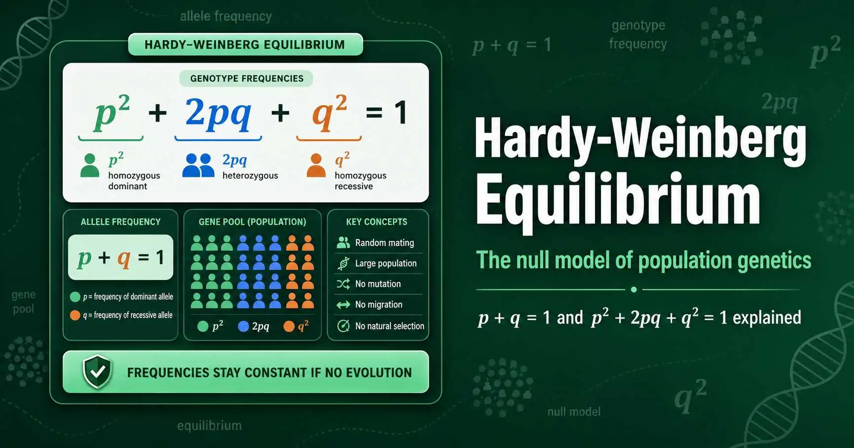
Hardy-Weinberg equilibrium is a principle stating that allele and genotype frequencies in a population stay constant from one generation to the next, as long as no evolutionary forces act on it. It is captured by two equations: p + q = 1 for allele frequencies, and p² + 2pq + q² = 1 for genotype frequencies. When a population meets the required conditions, these frequencies do not change, which makes the principle the baseline that population genetics measures everything against.
The idea sounds abstract, but it answers a question that puzzled early geneticists: why does a dominant allele not gradually take over a population and wipe out the recessive one? Hardy-Weinberg shows that, on its own, inheritance does not change allele frequencies at all. This guide explains what the equilibrium means, what each equation tells you, the conditions a population must meet, and why the principle is so central to studying evolution. The equations can be applied to real data with a calculator, but understanding the concept first makes the numbers meaningful.
The Core Idea: Frequencies That Stay Constant
At its heart, Hardy-Weinberg equilibrium describes a population that is not evolving. In such a population, the proportions of each allele and each genotype remain steady generation after generation, frozen in place by the absence of any force that would change them. Nothing drifts, nothing is selected for or against, and the genetic makeup simply reproduces itself, an idealized stillness that no real population perfectly achieves but many approximate closely enough to be useful.
This was a genuinely surprising result when Godfrey Hardy and Wilhelm Weinberg independently worked it out in 1908. Many people assumed that a dominant allele, because it masks the recessive one, would slowly become more common until the recessive allele vanished. Hardy and Weinberg proved this assumption wrong. Dominance describes how alleles interact within an individual, not how common they are in a population. By itself, the shuffling of alleles during reproduction does not favor one allele over another, so their frequencies stay put.
The principle works because of a simple but powerful logic. If you know the frequencies of the alleles in one generation, and nothing disturbs them, you can predict the genotype frequencies in the next generation exactly. Those genotype frequencies then produce the same allele frequencies again, which produce the same genotypes, and so on indefinitely. The population settles into a stable distribution that perpetuates itself. This self-sustaining constancy is what the word equilibrium captures, and it is the foundation everything else builds on.
A Question That Puzzled Early Geneticists
It helps to know the problem Hardy-Weinberg was invented to solve, because the principle answers a real confusion that troubled biologists in the early 1900s. After Mendel's work was rediscovered, a puzzle emerged about dominant traits in populations.
The worry went like this. If a dominant allele produces a 3:1 ratio in a cross, and dominance somehow gives an allele an advantage, then surely the dominant allele should spread through a population until the recessive one disappears entirely. Some prominent scientists of the era believed exactly this, expecting dominant traits to inevitably become universal. The question was sharp: if a gene pool starts with, say, 70 percent of one allele and 30 percent of another, what stops the more common or dominant allele from taking over completely over the generations?
Godfrey Hardy, an English mathematician, and Wilhelm Weinberg, a German physician, answered this independently in 1908. Their insight was that, in the absence of disturbing forces, allele frequencies do not change at all from one generation to the next. The 70-30 split stays 70-30. Dominance determines which allele is expressed in a heterozygote, but it has no power to change how often the allele appears in the gene pool. Reproduction reshuffles alleles into new individuals, but it does not alter their proportions. This resolved the puzzle and, in doing so, gave population genetics its founding principle. That a mathematician and a physician arrived at the same result separately, in the same year, underscores how fundamental the relationship is.
The First Equation: p + q = 1
The first Hardy-Weinberg equation deals with allele frequencies, and it is almost self-evident once you see it. For a gene with two alleles, the frequency of one allele plus the frequency of the other must add up to 1, or 100 percent, because together they account for every copy of that gene in the population.
By convention, p represents the frequency of the dominant allele and q represents the frequency of the recessive allele. So p + q = 1 simply says that all the dominant alleles plus all the recessive alleles make up the whole pool of alleles for that gene. If the dominant allele has a frequency of 0.7, then the recessive allele must have a frequency of 0.3, because the two have to total 1. This relationship lets you find one allele frequency the moment you know the other.
The idea of an allele frequency is worth pinning down clearly. It is the proportion of all the copies of a gene in a population that are a particular allele. Imagine pooling every allele from every individual into one big collection, often called the gene pool. The allele frequency is just the fraction of that pool made up by each version. Because every individual carries two alleles per gene, a population of 100 individuals has 200 alleles for a given gene, and p and q describe how those 200 are split. This simple counting idea is the starting point for every Hardy-Weinberg calculation.
The Second Equation: p² + 2pq + q² = 1
The second equation is the famous one, and it connects allele frequencies to genotype frequencies. It states that p² + 2pq + q² = 1, where each term gives the expected proportion of one genotype in the population. This is the equation that lets you predict how common each genotype will be.
Each term has a clear meaning. The p² term is the frequency of the homozygous dominant genotype, the individuals carrying two dominant alleles. The q² term is the frequency of the homozygous recessive genotype, those with two recessive alleles. The 2pq term is the frequency of the heterozygous genotype, the individuals with one of each allele. The reason heterozygotes get a factor of 2 is that they can form in two ways: the dominant allele from the mother and recessive from the father, or the reverse. Adding the three genotype frequencies together accounts for the entire population, so they sum to 1.
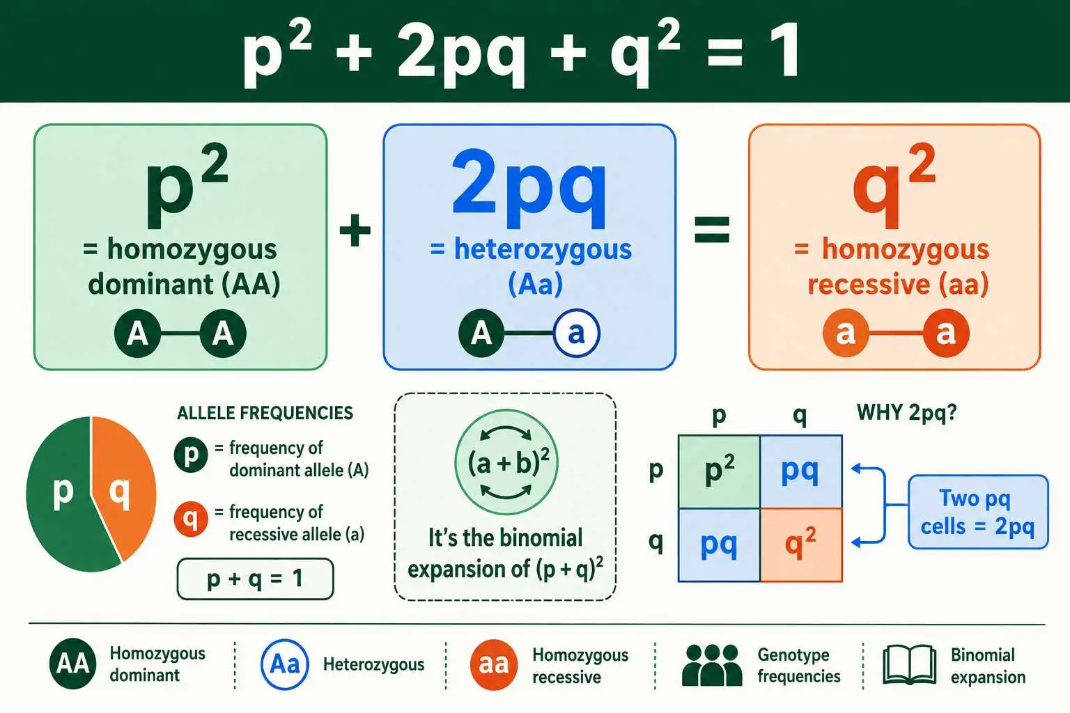
This equation is not arbitrary; it is the binomial expansion of (p + q)². Squaring p + q gives p² + 2pq + q², which is exactly the genotype equation. This makes sense because forming a diploid individual means drawing two alleles from the gene pool, and the chance of each combination follows the same math as multiplying out (p + q)². In effect, the equation applies the probability rules of a Punnett square to a whole population at once, predicting genotype proportions from allele frequencies. Understanding the link between genotype and the underlying alleles is easier with a grasp of genotype versus phenotype, which underpins the whole framework.
How the Two Equations Work Together
The two equations are a matched pair, and using them together is what makes Hardy-Weinberg so useful. One handles alleles, the other handles genotypes, and you can move between them depending on what information you start with. This flexibility is the practical heart of the principle.
The most common real-world starting point is the homozygous recessive genotype, because it is the one you can often count directly. Recessive conditions show up only in individuals with two recessive alleles, the q² group, so their frequency in a population gives you q² straight away. From there, you take the square root to find q, the recessive allele frequency. Then p + q = 1 gives you p, the dominant allele frequency. Finally, p² and 2pq give you the frequencies of the homozygous dominant and heterozygous genotypes. A single observable number, the proportion of affected individuals, unlocks the entire genetic structure of the population.
This chain of reasoning is the engine behind most Hardy-Weinberg problems. Start with what you can observe, usually q², work back to the allele frequencies, then forward to all the genotype frequencies. The two equations form a complete system: knowing the alleles tells you the genotypes, and knowing certain genotypes tells you the alleles. The detailed steps of running this calculation are covered in our guide on how to use the Hardy-Weinberg equation, but the key insight is that the two equations let you reconstruct an entire population's genetics from limited data. This is especially valuable because allele frequencies themselves are hard to measure directly, you cannot easily look at a person and read off which alleles they carry, but the frequency of an observable condition is often a matter of public health record. The equations turn that one accessible number into a full genetic profile of the population.
The Five Conditions for Equilibrium
Hardy-Weinberg equilibrium holds only when a population meets five specific conditions. These are the assumptions baked into the model, and they describe a population experiencing none of the forces that cause evolution. Real populations rarely meet all five perfectly, which is precisely what makes the principle useful as a comparison.
The five conditions are: a large population size, random mating, no mutation, no migration, and no natural selection. A large population prevents random chance from shifting allele frequencies, an effect called genetic drift that matters most in small populations. Random mating means individuals pair without regard to genotype, so no genotype gets a reproductive head start. No mutation means alleles are not being changed into other alleles. No migration means no individuals enter or leave to add or remove alleles. And no natural selection means every genotype survives and reproduces equally well, with no fitness advantage for any allele.
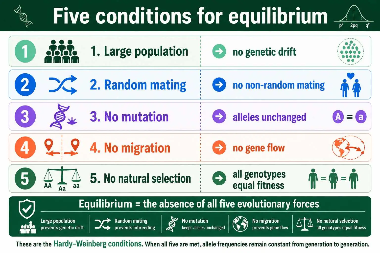
Each condition corresponds to a known force of evolution, which is the deeper point. Genetic drift, non-random mating, mutation, gene flow, and selection are exactly the processes that change allele frequencies over time. Hardy-Weinberg equilibrium is simply the state where none of them is operating. Because the conditions and what disrupts them are so central, we cover them in depth in our guide to the five assumptions of Hardy-Weinberg. For now, the essential idea is that equilibrium is the absence of evolution, defined by the absence of these five forces.
Why It Matters: The Null Model of Evolution
The single most important use of Hardy-Weinberg equilibrium is as a null model, a baseline of what a non-evolving population looks like. Scientists do not expect real populations to be in perfect equilibrium. Instead, they use the equilibrium prediction as a yardstick, and the interesting biology lies in how real data deviate from it.
The logic is the same as in statistics, where a null hypothesis represents no effect, and you look for evidence against it. Hardy-Weinberg gives you the expected genotype frequencies if nothing evolutionary is happening. You then compare those expectations against the genotype frequencies actually observed in a population. If the observed numbers match the prediction, the population may not be evolving at that gene. If they differ significantly, something is changing the frequencies, pointing to one of the evolutionary forces at work.
This makes the principle a detective tool. A deviation from Hardy-Weinberg equilibrium is a signal that mutation, migration, drift, non-random mating, or selection is acting on the population. Population geneticists use this comparison constantly, testing whether genes are in equilibrium and, when they are not, investigating why. Far from being a description of how populations actually behave, Hardy-Weinberg is valuable precisely because real populations depart from it, and those departures reveal evolution in action. This is why the principle, despite describing an idealized situation that rarely exists, sits at the foundation of the entire field.
The comparison is more than conceptual; it can be made statistically rigorous. By counting the genotypes actually present in a sample and comparing them to the p², 2pq, and q² values the equation predicts, researchers can test mathematically whether a population departs from equilibrium. A small difference is treated as ordinary sampling noise, while a large one signals that an evolutionary force is at work. As the Fiveable genetics guide puts it, the equilibrium is the baseline you compare everything else against, which is exactly what makes it indispensable despite being an idealization.
What Equilibrium Does Not Mean
Because the word equilibrium suggests stability, it invites a few misconceptions worth clearing up. Understanding what Hardy-Weinberg does not claim is as important as understanding what it does, since these misunderstandings trip up many students.
The first misconception is that equilibrium means a population never changes or never evolves. The principle does not say that; it says a population will not change at a given gene only if the five conditions are met. Since real populations almost always violate at least one condition, they do evolve. Hardy-Weinberg describes a theoretical baseline, not a claim about reality. The second misconception is that dominant alleles should become more common over time. This is exactly the assumption Hardy and Weinberg disproved. Dominance affects how an allele is expressed, not how frequently it occurs, so a dominant allele does not increase in frequency just by being dominant.
A third misconception concerns the type of equilibrium. Hardy-Weinberg equilibrium is a neutral equilibrium, not a stable one. In a stable equilibrium, a system pushed away from its balance point returns to it, like a ball rolling back to the bottom of a bowl. Hardy-Weinberg is different. If something shifts the allele frequencies, the population does not return to its old frequencies; instead it settles into a new equilibrium at the new frequencies. The genotype proportions snap back into the p² : 2pq : q² pattern within one generation, but around whatever allele frequencies now exist. This distinction matters because it explains how allele frequencies can change permanently while genotype frequencies always realign to the predictable pattern.
A Simple Worked Example
A quick example shows the principle in action. Suppose a recessive condition affects 1 in 100 people in a population, and we want to know how many people carry the allele without being affected. This is the classic Hardy-Weinberg question.
Start with what you can observe. Affected individuals are homozygous recessive, the q² group, and they make up 1 in 100, or 0.01, of the population. So q² equals 0.01. Taking the square root gives q equals 0.1, the frequency of the recessive allele. Since p + q = 1, the dominant allele frequency p equals 0.9. Now you can find the genotype frequencies. The homozygous dominant frequency p² is 0.9 squared, which is 0.81. The heterozygous carrier frequency 2pq is 2 times 0.9 times 0.1, which is 0.18.
The result is striking. While only 1 percent of the population is affected, fully 18 percent are carriers, heterozygotes who carry the recessive allele but do not show the condition.
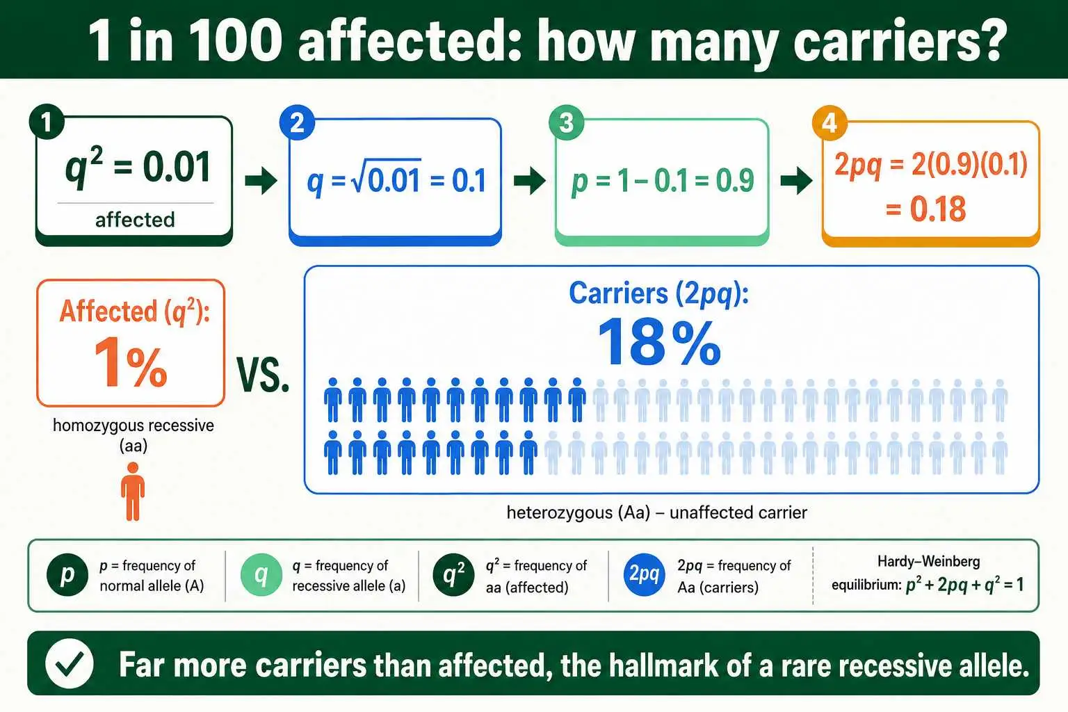
There are far more carriers than affected individuals, which is a general feature of rare recessive alleles, since q² is much smaller than 2pq when q is small. This single example demonstrates the power of the principle: from one observed number, the frequency of affected individuals, you reconstruct the entire genetic makeup of the population. It also explains why recessive alleles persist, hidden in carriers rather than exposed to selection. The distinction between these carrier heterozygotes and affected homozygotes rests on the difference between being homozygous versus heterozygous, which the genotype terms p², 2pq, and q² directly describe.
Frequently Asked Questions
What is Hardy-Weinberg equilibrium in simple terms?
It is the principle that allele and genotype frequencies in a population stay constant from generation to generation as long as no evolutionary forces act on it. It describes a population that is not evolving, serving as a baseline for detecting when evolution is occurring.
What do p and q stand for?
In the Hardy-Weinberg equations, p is the frequency of the dominant allele and q is the frequency of the recessive allele. Because a gene with two alleles has only these two options, p + q must equal 1, accounting for all copies of the gene.
What does p² + 2pq + q² = 1 mean?
It gives the expected genotype frequencies in a population. The p² term is the homozygous dominant frequency, 2pq is the heterozygous frequency, and q² is the homozygous recessive frequency. Together they account for everyone, so they sum to 1.
Why is Hardy-Weinberg equilibrium important if no population is really in it?
Because it serves as a null model. Scientists compare real populations against the equilibrium prediction, and deviations reveal that evolutionary forces like selection, drift, or migration are at work. Its value lies in detecting evolution, not describing reality.
The Takeaway
Hardy-Weinberg equilibrium is the principle that a population's allele and genotype frequencies stay constant across generations when no evolutionary forces disturb it. Its two equations, p + q = 1 for alleles and p² + 2pq + q² = 1 for genotypes, let you predict the genetic makeup of a population from limited data, most often by starting with the observable frequency of a recessive condition and working backward to the alleles. The principle holds only when five conditions are met: large population, random mating, no mutation, no migration, and no selection.
Its real power is as the null model of population genetics. Because real populations deviate from equilibrium, those deviations become a way to detect and study evolution itself. You can run the calculations for any population with the Hardy-Weinberg allele frequency calculator, which applies both equations to your data instantly. For a rigorous academic treatment of the principle, this overview from Nature Education is a thorough and reliable reference.