LD Decay and Recombination Explained
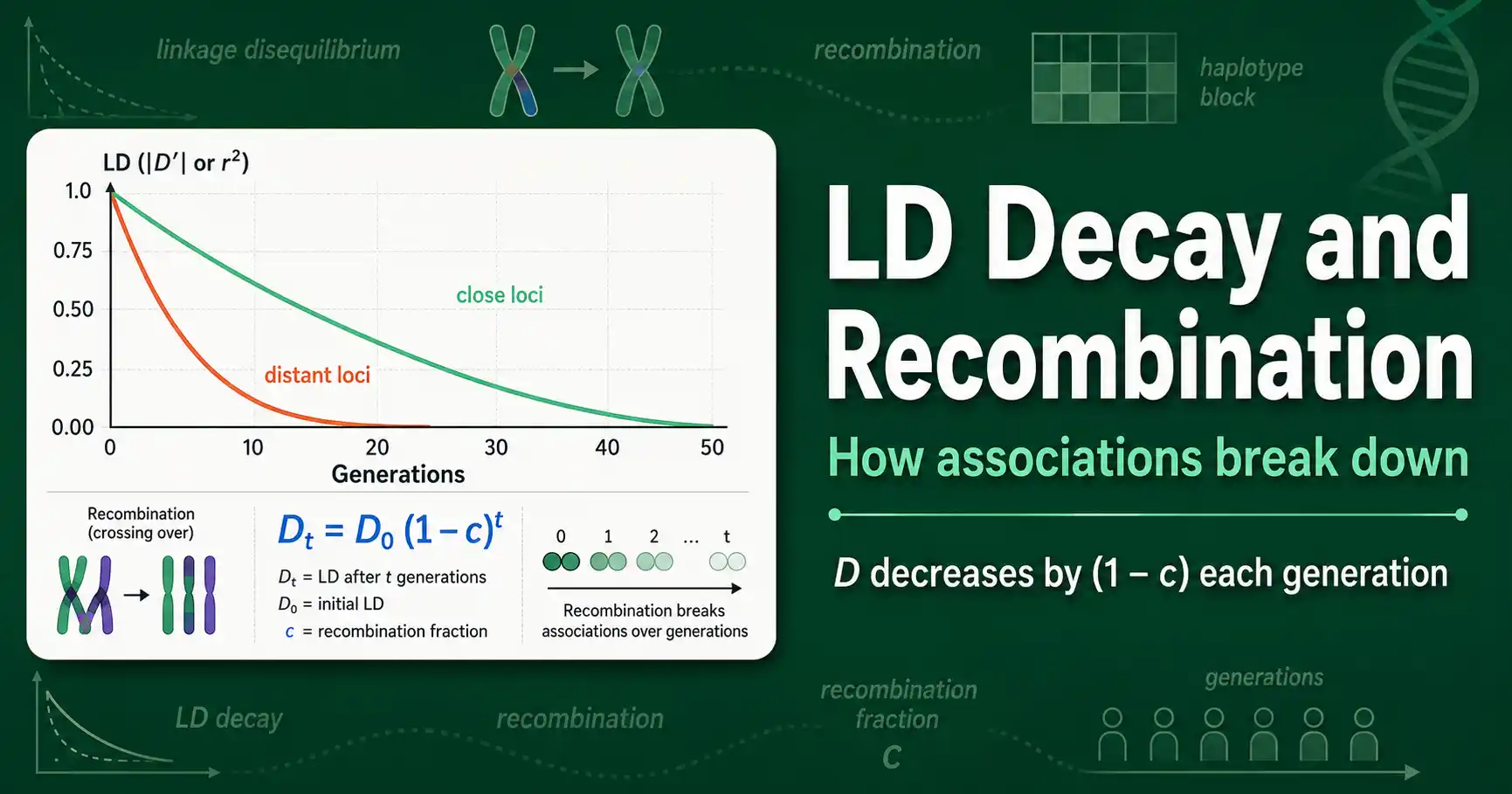
Linkage disequilibrium decays over time because recombination keeps shuffling alleles between chromosomes, breaking the associations between loci. The closer two loci sit, the slower their LD decays, because recombination rarely separates them. The farther apart they are, the faster it fades. This decay, set by recombination, is what shapes the LD structure of every genome.
This guide explains how LD breaks down. It covers the decay formula, why physical distance governs the rate, how recombination hotspots carve the genome into haplotype blocks, and why population history leaves its mark on the pattern. For the foundation, our explainer on what linkage disequilibrium is sets up the concept.
Recombination Breaks LD Down
Recombination is the force that erodes linkage disequilibrium. Each generation, when chromosomes pair and exchange segments during meiosis, recombination can separate alleles that were traveling together, nudging the loci toward independence.
Here is the mechanism. Suppose alleles A and B sit together on one chromosome, in LD. If a recombination event occurs between their two loci, the offspring chromosome may carry A with b instead, breaking the original association. Every generation, some fraction of chromosomes recombine between the loci, and each such event chips away at the LD. Left to run, recombination drives any pair of loci toward linkage equilibrium, where the alleles are independent.
The speed of this breakdown depends entirely on how often recombination happens between the two loci, which in turn depends on how far apart they are. That single fact, recombination rate set by distance, governs nearly everything about LD decay.
Crossover recombination is the main eraser, but it is not the only one. Gene conversion, a process that copies a short stretch of sequence from one chromosome onto its homolog without exchanging the flanking regions, also breaks down LD, and it acts over very short distances. For loci just a few hundred base pairs apart, gene conversion can be a more important cause of LD breakdown than crossover recombination. This is why LD does not always rise smoothly to its maximum at the very shortest distances: the finest-scale associations are eroded by conversion even where crossovers are rare. For most purposes, though, crossover recombination is the dominant force, and the decay formula captures its effect well.
The Decay Formula
LD decays geometrically, losing a constant fraction of its value each generation. The formula is simple and worth knowing.
The linkage disequilibrium after t generations equals the starting LD times the quantity one minus c, raised to the power t:
D_t = D_0 × (1 − c)^t
Here D_0 is the initial LD, c is the recombination fraction between the loci, and t is the number of generations. The recombination fraction c is the probability that recombination separates the two loci in a single generation, ranging from zero for loci right next to each other to one-half for loci that assort independently.
Work through what this implies. For unlinked loci, where c is one-half, LD halves every generation, so it vanishes almost immediately. For tightly linked loci, where c is tiny, the term one minus c is close to one, so LD barely shrinks each generation and can persist for hundreds or thousands of generations. This is the mathematical heart of why nearby loci stay associated while distant ones do not. The decay is exponential in time and steep in recombination rate.
Distance Sets the Rate
Because the recombination fraction tracks physical distance along the chromosome, distance is what ultimately controls how fast LD decays. This produces the signature pattern seen in every genome.
Loci close together recombine rarely, so c is small, and their LD persists across many generations. Loci far apart recombine often, so c is large, and their LD decays quickly. Plot LD against distance and you get the classic LD decay curve: high near zero distance, falling off as separation grows. The exact shape of that curve, how quickly LD drops with distance, is a property of each population and each genomic region.
This distance dependence is what makes LD useful for mapping. If a marker is in strong LD with a nearby variant, the two are likely close together, so finding a marker associated with a disease points to a nearby causal region. The table below shows how the recombination fraction shapes persistence.
It helps to keep physical distance and genetic distance separate here. Physical distance, measured in base pairs, is not a perfect guide to recombination, because recombination rate varies along the chromosome. Genetic distance, measured in centimorgans, is defined directly by recombination: one centimorgan corresponds to a one percent chance of recombination per generation. LD decay tracks genetic distance, not physical distance, which is why two loci the same number of base pairs apart can show very different LD depending on whether a recombination hotspot sits between them. When people say LD decays with distance, the distance that truly matters is the genetic one.
| Recombination fraction (c) | Loci relationship | LD persistence |
|---|---|---|
| 0.5 | Unlinked or far apart | Halves every generation, gone fast |
| 0.1 | Loosely linked | Decays over tens of generations |
| 0.01 | Closely linked | Persists for many generations |
| 0.001 | Very tightly linked | Persists for thousands of generations |
The pattern is consistent: smaller recombination fractions, meaning closer loci, mean slower decay and longer-lasting LD. You can explore how a given recombination fraction erodes an initial LD value over generations by running the decay numbers through an LD tool alongside the formula.
A Worked Decay Example
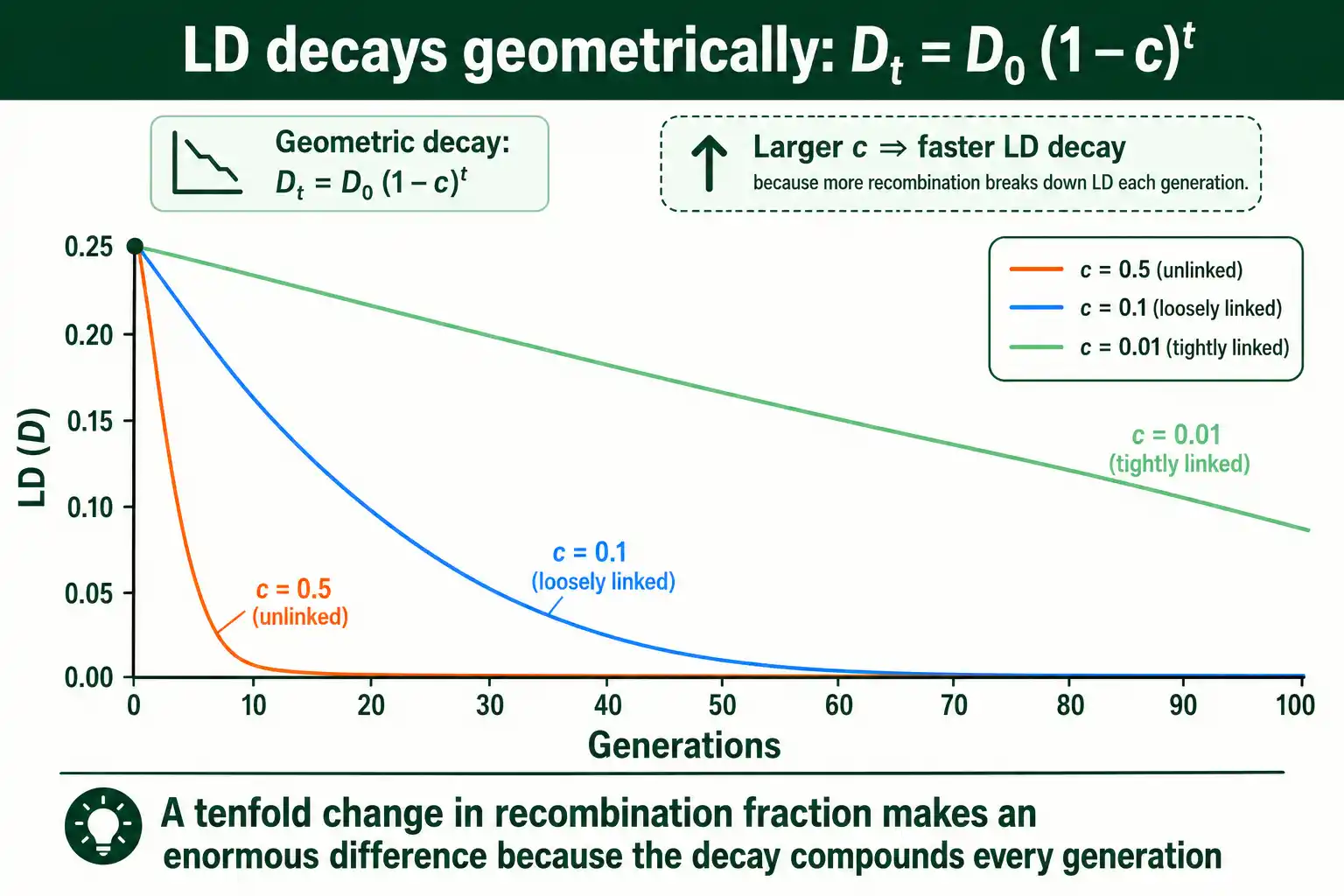
Numbers make the formula concrete. Start with two loci in strong association, an initial D of 0.25, and follow what happens at different recombination fractions over generations.
Take loosely linked loci with a recombination fraction of 0.1. After one generation, D is 0.25 times 0.9, or 0.225. After five generations, it is 0.25 times 0.9 to the fifth power, about 0.148. After twenty generations, it is down to roughly 0.030. The LD is clearly fading, but it takes dozens of generations to approach zero.
Now compare tightly linked loci with a recombination fraction of 0.01. After one generation, D is 0.25 times 0.99, or 0.2475, barely changed. After twenty generations it is still about 0.204, having lost less than a fifth of its value. After a hundred generations it remains near 0.092. The same starting LD persists vastly longer simply because recombination separates these loci ten times less often.
The contrast captures the whole principle. A tenfold difference in recombination fraction produces an enormous difference in how long LD survives, because the effect compounds every generation. This is why a snapshot of LD across a genome is effectively a map of recombination rates: the loci still in strong LD are the ones recombination has left alone.
Measuring the Extent of LD
Researchers summarize how far LD reaches in a region or population with a measure called the extent of LD, usually the distance over which average LD, measured by r squared, falls below some threshold. It is a practical shorthand for how quickly associations break down.
In humans, LD typically extends over tens of kilobases before r squared drops to low levels, though this varies widely by region and population. In species with smaller effective population sizes, or in domesticated crops and livestock shaped by intense recent breeding, LD often extends much farther, sometimes over megabases. The extent of LD directly sets how densely a genome must be genotyped for association mapping: short-range LD demands many markers, while long-range LD lets fewer markers cover the same ground.
This is why the extent of LD is one of the first things measured when planning a genome-wide study in any species. A population with long-range LD needs a sparser marker panel, lowering cost, but also yields coarser mapping resolution, since each associated marker implicates a larger region. The trade-off between marker density and resolution traces directly back to how fast LD decays.
Recombination Is Not Uniform
A crucial complication: recombination does not happen evenly along the chromosome. It clusters in narrow regions called recombination hotspots, with long stretches of low recombination in between. This unevenness shapes LD profoundly.
Fine-scale recombination maps of the human genome, generated by Simon Myers and colleagues in a 2005 Science paper, revealed enormous variation in recombination rate. Hotspots can reach rates of 10 to 60 centimorgans per megabase, while the regions between them sit close to zero. Most recombination is concentrated in these hotspots, which occupy a small fraction of the genome.
The consequence for LD is striking. Within the low-recombination regions between hotspots, alleles stay associated for long stretches, producing strong LD. At the hotspots, recombination rapidly breaks LD down. So the genome's LD is not a smooth gradient but a series of high-LD regions punctuated by sharp breakdowns. This structure has a name, and it changed how human genetics is done.
Haplotype Blocks
The uneven recombination landscape carves the genome into haplotype blocks: regions of strong internal LD where only a few haplotypes are common, separated by the recombination hotspots where LD breaks down. This block structure was a major finding of early genomic studies.
The picture emerged from work by Stacey Gabriel and colleagues in a 2002 Science paper, which showed that human DNA is organized into blocks of limited haplotype diversity, bounded by short regions of historical recombination. Within a block, the loci are in high LD, so only a handful of haplotype combinations actually occur, far fewer than the number theoretically possible. Between blocks, recombination has mixed the alleles freely.
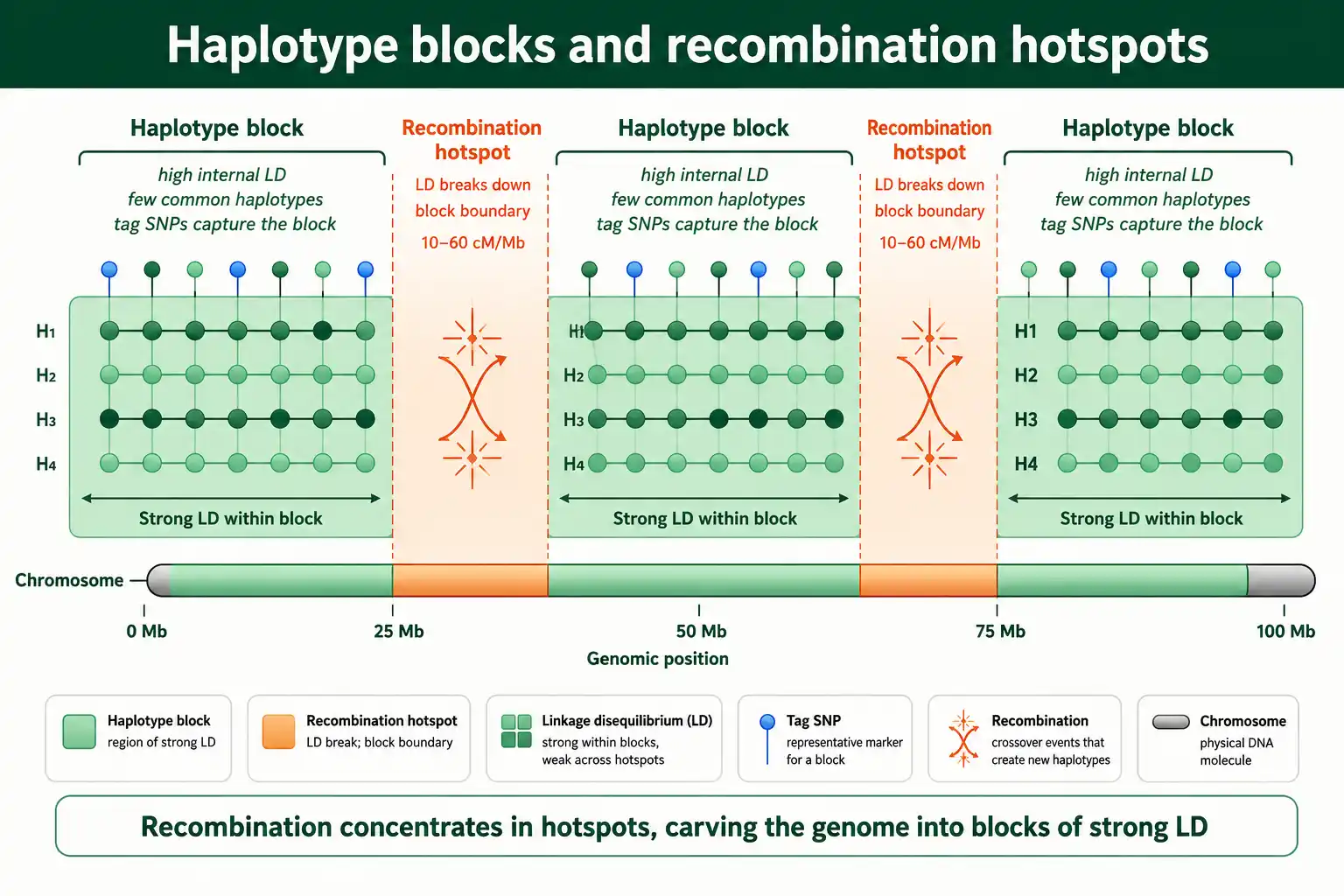
This block structure is the foundation of efficient genotyping. Because the loci within a block are highly correlated, you do not need to genotype every variant; a few well-chosen tag SNPs capture most of the variation in the block. This insight made genome-wide association studies practical, since it meant a few hundred thousand tag SNPs could represent the common variation across the whole genome. The block structure also explains why an associated marker points to a block-sized region rather than a single base, which is why fine-mapping is needed afterward, a theme in our guide on linkage disequilibrium in GWAS.
The boundaries between blocks are not arbitrary. They sit where recombination hotspots have repeatedly broken associations, so the same boundaries tend to recur across individuals and even, partly, across related populations. This recurrence is what lets researchers build a shared map of haplotype blocks for a population rather than re-deriving them for every study. The international HapMap project did exactly this, cataloguing common haplotype blocks and the tag SNPs that capture them across several human populations, which became the scaffolding for a generation of association studies. The deep point is that the LD map and the recombination map are two views of the same thing: wherever recombination is rare, LD is strong and blocks form; wherever it is intense, LD collapses and a boundary appears.
Population History Shapes Decay
The rate of LD decay is not set by recombination alone. A population's history, especially its size and any bottlenecks, leaves a strong imprint, which is why LD patterns differ between populations.
The link runs through genetic drift. In a small population, drift is strong and constantly generates new LD by chance, which counteracts recombination's breakdown and lets LD extend over longer distances. In a large population, drift is weak, so recombination wins and LD decays over shorter distances. This is why small or recently bottlenecked populations show longer-range LD and larger haplotype blocks than large, stable ones.
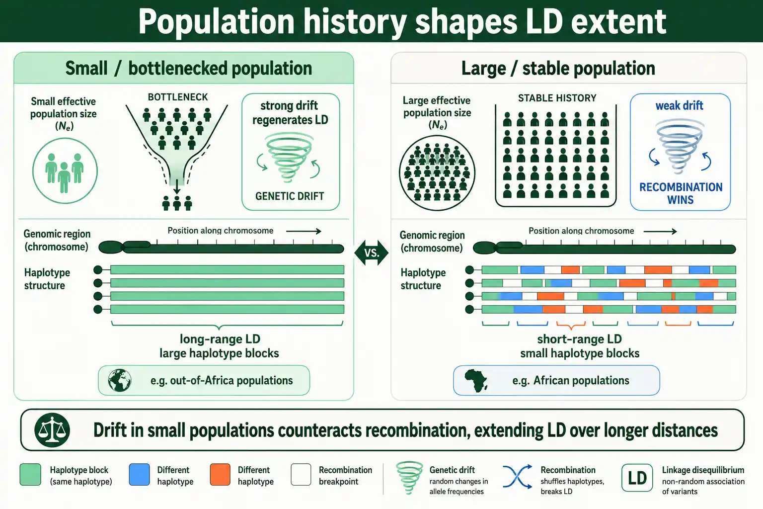
Human populations illustrate this directly. Because non-African populations passed through the out-of-Africa bottleneck, they have larger haplotype blocks and more extensive LD than African populations, which retained larger effective sizes and so show shorter-range LD. The connection between population size and LD runs deep enough that LD decay patterns are used in reverse, to estimate a population's historical effective size and reconstruct events like bottlenecks and expansions. This bridge to drift and population size is developed in our guide on effective population size, and the broader set of forces is covered in our guide on what causes linkage disequilibrium.
The logic of the reverse inference is elegant. LD between loci at a given recombination distance reflects, roughly, the population size some number of generations ago, with closer loci carrying information about deeper history and distant loci about recent history. By measuring how r squared declines with recombination distance, researchers can read off an effective-size trajectory through time: a dip in the inferred size at a particular era flags a past bottleneck, a rise flags an expansion. This LD-based demographic inference has reconstructed the timing of the out-of-Africa bottleneck and later population expansions from present-day genomes alone, without any ancient DNA. It is one of the clearest examples of LD serving as a record of the past rather than just a tool for the present.
Frequently Asked Questions
Why does linkage disequilibrium decay over time?
Because recombination shuffles alleles between chromosomes each generation, breaking the associations between loci. Every generation, some fraction of chromosomes recombine between two loci, separating alleles that were traveling together, so the LD shrinks. Over enough generations, recombination drives the loci toward linkage equilibrium unless some force keeps regenerating the association.
What is the formula for LD decay?
LD decays geometrically: D after t generations equals the starting LD times one minus c, raised to the power t, where c is the recombination fraction between the loci. For unlinked loci, c is one-half and LD halves each generation. For tightly linked loci, c is tiny, so LD barely shrinks per generation and persists for a very long time.
What is a haplotype block?
A haplotype block is a region of the genome with strong internal linkage disequilibrium, where only a few haplotypes are common, bounded by recombination hotspots where LD breaks down. Within a block, loci are highly correlated, so a few tag SNPs capture most of the variation, which is the basis of efficient genome-wide genotyping.
The Balance of Building and Breaking
Linkage disequilibrium decays because recombination keeps separating associated alleles, and the rate of decay follows a simple geometric formula governed by the recombination fraction between loci. Since that fraction tracks physical distance, nearby loci hold their LD for many generations while distant ones lose it fast, producing the LD decay curve at the center of gene mapping.
Recombination is not uniform, though. It concentrates in hotspots, carving the genome into haplotype blocks of strong internal LD separated by sharp breakdowns, the structure that made tag-SNP genotyping and modern association studies possible. And because drift in small populations regenerates LD, population history leaves its signature in how far LD extends, with bottlenecked populations showing larger blocks. The recombination that tears LD down is only half the story; the forces that build it are the other half.