What Is Linkage Disequilibrium? (LD Explained)
Linkage disequilibrium, or LD, is the non-random association of alleles at different genetic loci. When two alleles at separate loci show up together more often, or less often, than chance would predict, they are in linkage disequilibrium. When they occur together exactly as often as their individual frequencies predict, they are in linkage equilibrium.
That is the whole idea: LD measures whether the alleles you carry at one spot in the genome tell you anything about which alleles you carry at another spot. This guide explains what LD is, how it differs from genetic linkage, what creates it, and why it has become central to modern genetics. The concept builds on the independence that Hardy-Weinberg assumes, covered in our guide on Hardy-Weinberg equilibrium.
The Core Idea
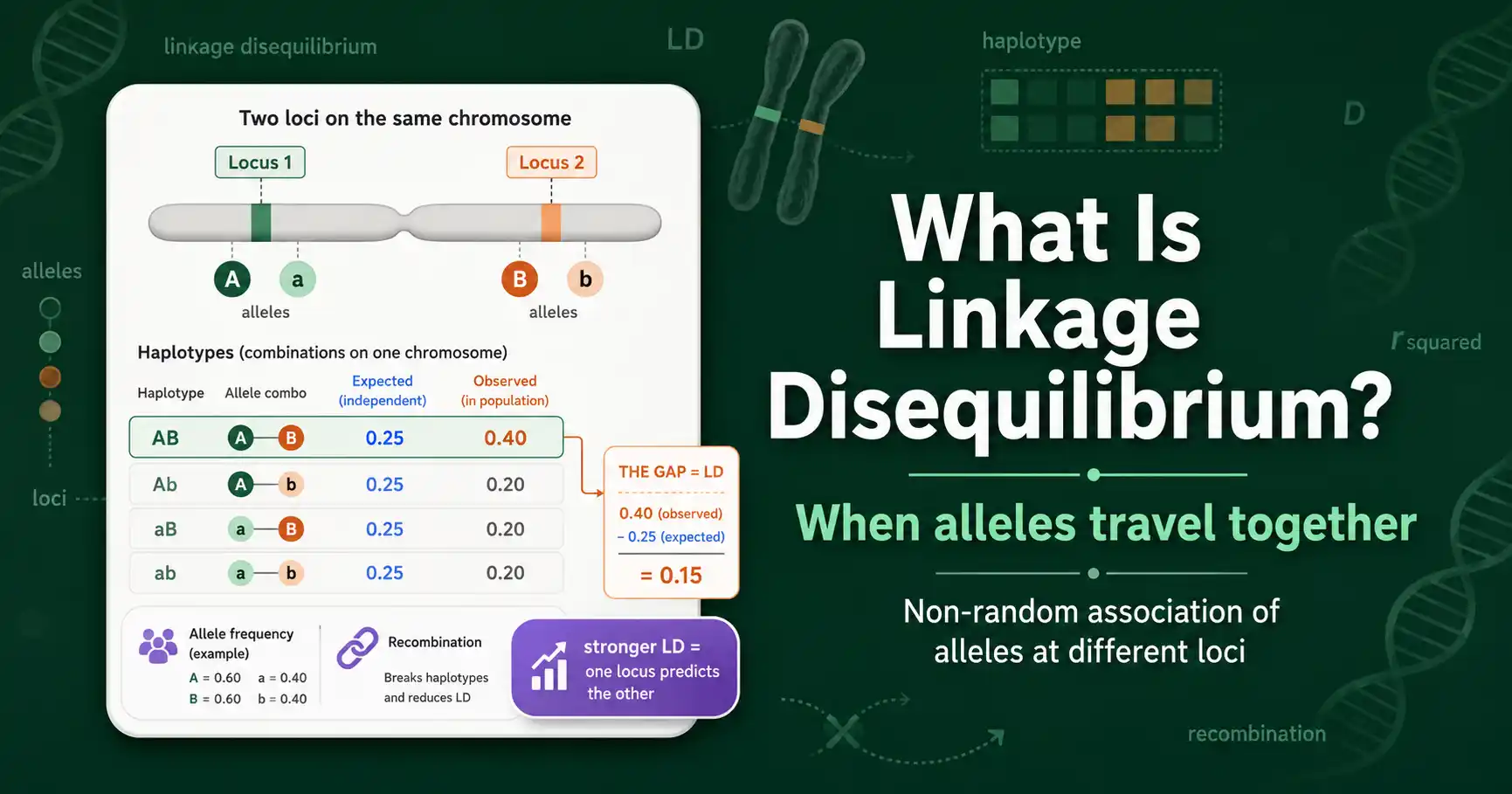
Picture two genes on a chromosome. The first has alleles A and a; the second has alleles B and b. Across a population, each allele has some frequency. If the alleles combine randomly, the frequency of any haplotype, say AB, is simply the product of the two allele frequencies.
Linkage disequilibrium is the gap between that expectation and reality. If AB appears more often than the product of A's frequency and B's frequency, then A and B are associated, and LD is present. The alleles are traveling together through generations more than chance allows. If the haplotype frequencies match the products exactly, there is no association, and the loci are in equilibrium.
So LD is really a statement about predictability. Under linkage equilibrium, knowing someone's allele at the first locus tells you nothing about their allele at the second. Under linkage disequilibrium, it tells you something, because the alleles are correlated. The stronger the LD, the more reliably one locus predicts the other, all the way up to perfect prediction when the association is complete.
A Concrete Example
Numbers make this tangible. Suppose allele A has a frequency of 0.5 and allele B has a frequency of 0.5. If the two loci are independent, the AB haplotype should appear at 0.5 times 0.5, which is 0.25, a quarter of the time.
Now suppose you actually count haplotypes and find AB at 0.4, not 0.25. That excess is linkage disequilibrium. A and B are turning up together more than chance predicts, so the loci are associated. Knowing someone carries A now makes it likelier they also carry B, which would be impossible under independence.
Flip it the other way and the same logic holds. If AB showed up at only 0.10, well below the expected 0.25, that is also LD, just in the opposite direction: A and B avoid each other. Either way, any departure from the expected product, in either direction, is linkage disequilibrium. The size of that gap is what the LD statistics measure.
Linkage Is Not Linkage Disequilibrium
The names cause endless confusion, so this distinction is worth making early. Linkage and linkage disequilibrium are related but different, and one does not require the other.
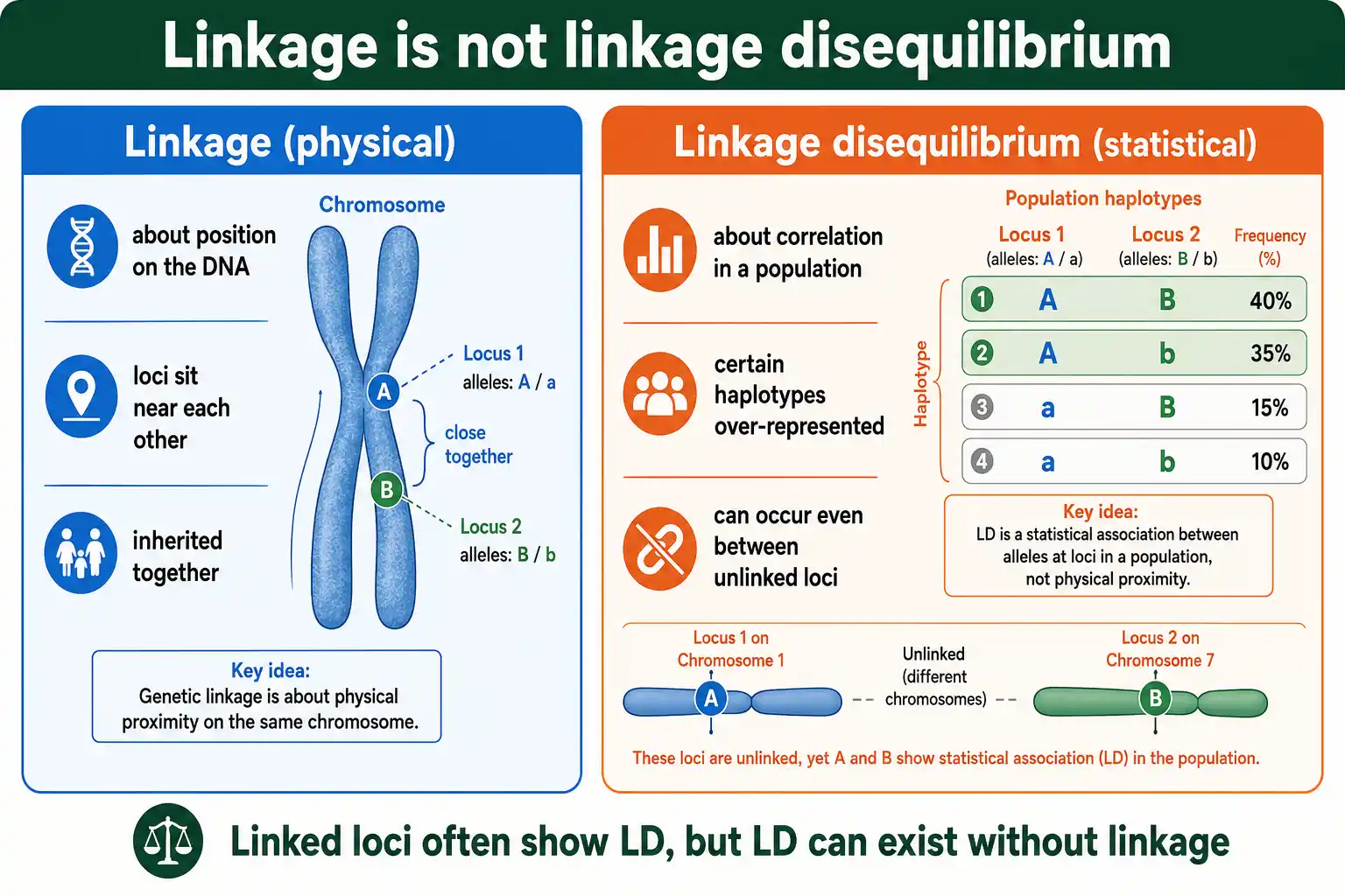
Genetic linkage is physical: two loci are linked when they sit close together on the same chromosome, so they tend to be inherited together because recombination rarely separates them. Linkage is about location on the DNA.
Linkage disequilibrium is statistical: it is a correlation between alleles in a population, regardless of where the loci sit. Linked loci often show LD, because their physical closeness keeps their alleles associated. But LD can also exist between loci on entirely different chromosomes, which are not linked at all, if some force other than proximity has correlated them. As Montgomery Slatkin noted in an influential 2008 review in Nature Reviews Genetics, linkage disequilibrium is one of those terms whose name actively hides its meaning, because the "linkage" in the name is not required for the phenomenon. The lesson is simple: linkage is about physical position, LD is about statistical association, and you can have one without the other.
How LD Is Measured
LD is quantified with a statistic called D, the simplest measure, introduced when the concept was formalized. D is the difference between the observed frequency of a haplotype and the frequency expected if the alleles were independent.
Written out, D equals the frequency of the AB haplotype minus the product of the frequency of A and the frequency of B. When D is zero, the alleles are independent and the loci are in linkage equilibrium. When D is not zero, LD is present, and the larger its absolute value, the stronger the association. The statistic was defined by Richard Lewontin and Ken-ichi Kojima in their 1960 paper, the work that coined the term linkage disequilibrium itself.
D has a drawback: its range depends on the allele frequencies, so a raw D value is hard to interpret on its own. To fix this, geneticists use two normalized measures. D prime, also from Lewontin, scales D by its maximum possible value given the allele frequencies, producing a number from negative one to one. The other is r squared, the squared correlation between the two loci, which runs from zero to one and is the measure most used in modern genomics. You can work through haplotype data and get D, D prime, and r squared with a linkage disequilibrium calculator.
These two normalized measures answer slightly different questions, which is why both survive. D prime of one means no recombination has yet separated the two loci in the sample, a sign of shared history, even if the alleles are not strongly correlated. R squared of one is stronger: it means the two loci are perfectly correlated, so one allele perfectly predicts the other. Because GWAS depends on one marker standing in for another, r squared, the measure of predictability, is the one association studies care about most. The difference between them is the subject of our guide on D prime versus r squared.
What Creates LD
If recombination constantly shuffles alleles, why does LD exist at all? Several forces generate it faster than recombination can erase it. Each leaves its own signature.
Physical linkage is the most common cause. Loci close together on a chromosome are rarely separated by recombination, so their alleles stay associated for many generations. The closer the loci, the stronger and longer-lasting the LD, which is why a genome's LD largely mirrors its physical map: neighbors are correlated, distant loci are not.
Other forces create LD even between distant or unlinked loci. Genetic drift generates LD by chance in finite populations, especially small ones. Natural selection generates it when it favors particular allele combinations, or when a beneficial allele sweeps and drags neighboring alleles with it. Population admixture, the recent mixing of two genetically different groups, creates strong LD because each source group brought its own allele combinations. New mutations start out in complete LD with everything around them, since a mutation arises on one specific haplotype. Each of these forces leaves a distinct LD signature, which is what makes LD such a rich record of a population's past.
What Breaks LD Down
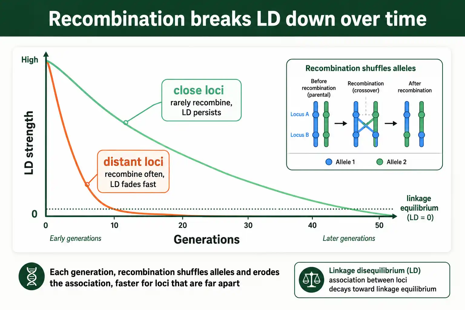
The force working against all of this is recombination. Each generation, recombination shuffles alleles between homologous chromosomes, gradually breaking up associations between loci.
The rate of breakdown depends on distance. Loci far apart recombine often, so their LD decays quickly, within a few generations. Loci very close together recombine rarely, so their LD persists for many generations. This is why LD in a genome tends to be strongest between nearby loci and fades with distance, a pattern called LD decay. Over enough time, recombination drives any pair of loci toward linkage equilibrium unless some force keeps regenerating the association.
This tug of war, forces building LD and recombination tearing it down, sets the LD structure of every genome. The balance is the subject of our guide on LD decay and recombination.
Why LD Matters
LD might sound abstract, but it underpins much of modern genetics. Three uses show why it matters.
The first is disease gene mapping. Genome-wide association studies, the workhorse of human genetics, rely on LD entirely. Researchers genotype a set of marker SNPs, and because each marker is in LD with nearby variants, a marker associated with a disease points to a nearby causal variant even if the marker itself is not the cause. This is what lets a study test a few hundred thousand markers and still capture variation across the whole genome: each marker tags the variants around it. Without LD, every causal variant would have to be genotyped directly, and association studies as we know them would be impossible.
The second is reconstructing population history. Because drift, admixture, and selection all leave LD signatures, the LD patterns in a genome record a population's past, its size changes, mixing events, and episodes of selection. Reading LD backward reveals that history.
The third is detecting natural selection. When a beneficial allele sweeps through a population, it drags neighboring alleles with it, creating a long stretch of strong LD. Scanning the genome for these unusually long, high-LD haplotypes is a standard way to find genes that have been under recent selection. These applications, especially in human genetics, are the focus of our guide on linkage disequilibrium in GWAS.
Frequently Asked Questions
What is the difference between linkage and linkage disequilibrium?
Linkage is physical: two loci are linked when they sit close together on the same chromosome and tend to be inherited together. Linkage disequilibrium is statistical: it is a non-random association between alleles in a population. Linked loci often show LD, but LD can also occur between unlinked loci on different chromosomes, so the two are not the same.
What does it mean when two loci are in linkage equilibrium?
It means their alleles are statistically independent. The frequency of any haplotype equals the product of the individual allele frequencies, so knowing the allele at one locus tells you nothing about the allele at the other. Linkage equilibrium is the absence of any association between the loci.
The Short Version
Linkage disequilibrium is the non-random association of alleles at different loci, the degree to which one locus predicts another. It is measured by D and its normalized forms, D prime and r squared, and it differs from genetic linkage, which is about physical position rather than statistical correlation. LD is built by linkage, drift, selection, admixture, and mutation, and broken down by recombination, with the balance between them shaping every genome.
The reason LD has moved to the center of genetics is practical. It powers genome-wide association studies, records population history, and reveals natural selection, all because the associations between alleles carry information. To see the math that turns haplotype frequencies into an LD value, the next step is our guide on how to calculate linkage disequilibrium.