How to Calculate the Inbreeding Coefficient

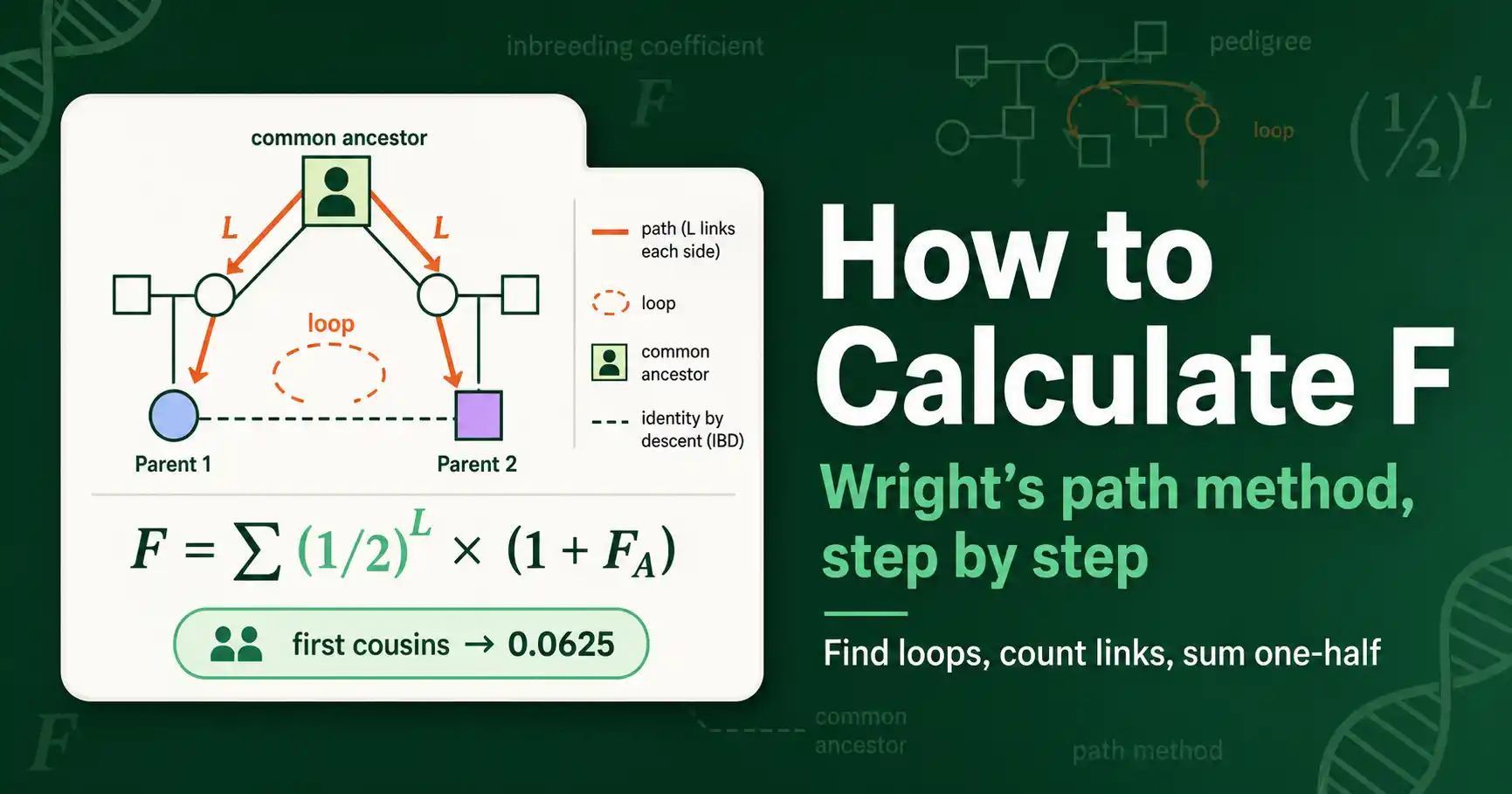
To calculate the inbreeding coefficient F, you trace the loops in a pedigree that connect an individual's two parents through their shared ancestors, then add up one-half raised to the length of each loop. That is the whole method. Everything else is detail.

This guide walks through it step by step. It covers the path-counting rule, three fully worked examples from simple to complex, the correction for ancestors who are themselves inbred, and the alternative method used for large breeding pedigrees. If you need the concept behind the number first, start with our explainer on what the inbreeding coefficient is.

The Method in Three Steps

Wright's path method, published in 1922, computes F from a pedigree in three steps. Learn these and you can do any standard pedigree.

Step one: find every common ancestor of the individual's two parents. A common ancestor is anyone who appears on both the mother's side and the father's side. These shared ancestors are the only source of inbreeding, because they are the only way the two parents can carry copies of the same ancestral allele.

Step two: for each common ancestor, trace the loop. A loop starts at one parent, goes up through ancestors to the common ancestor, then comes back down to the other parent. The rule that prevents mistakes: never pass through the same individual twice in a single loop. The number of separate loops equals the number of common ancestors.

Step three: count and sum. For each loop, count the number of links, the connecting lines between individuals from one parent up to the common ancestor and back down to the other parent. Raise one-half to that power. Add the results from all loops. That sum is F.

The formula, stated compactly, is F = Σ (1/2)^L, where L is the number of links in each loop and the sum runs over all loops. When a common ancestor is itself inbred, one extra factor applies, covered later. For now, the clean version carries most cases.

Before the worked examples, one orienting point. Every loop you trace is really following a single allele on its possible journey: down from a common ancestor through one parent to the child, and down again through the other parent. The (1/2) at each link is the Mendelian chance that the specific allele, not its alternative, was the one passed on. Multiplying those one-half chances along the whole loop gives the probability that the same ancestral allele reached the child twice, which is exactly identity by descent. Seeing the formula as a chain of coin-flip inheritance events, rather than an abstract rule, makes every step that follows intuitive. The same loop-tracing logic underlies reading any family chart, which our pedigree analyzer automates for inheritance patterns more broadly.

Worked Example 1: First Cousins

Start with the most common real case: the child of first cousins. The answer is 0.0625, and here is how it falls out.

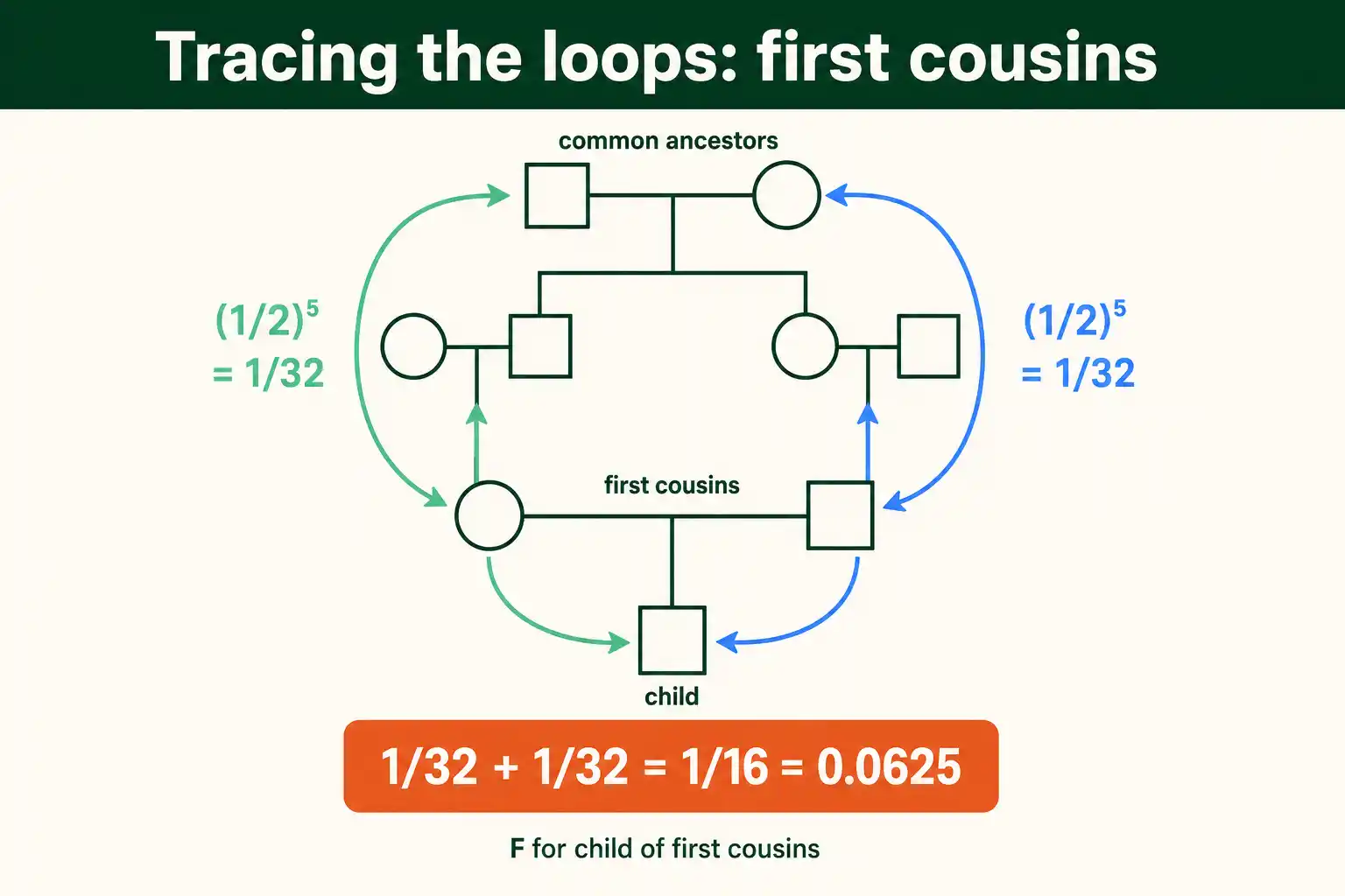
First cousins share two grandparents. Call the child X, the cousin parents are the mother and father, and the shared grandparents are the two common ancestors. So there are two loops, one through each grandparent.

Trace the loop through the first shared grandparent. From the mother, up to her parent (one link), up to the shared grandparent (a second link), then down to the father's parent (third link), then down to the father (fourth link). Counting the links from one parent through the grandparent and back gives a loop length of four on each side of that grandparent. Tracing carefully through the standard first-cousin pedigree, each of the two loops contributes (1/2) to the fifth power, which is 1/32.

Add the two loops: 1/32 plus 1/32 equals 1/16, which is 0.0625. That matches the textbook value for first cousins exactly. The method delivered the known answer, which is the point of starting here: it shows the procedure works on a case you can check.

Worked Example 2: Half Siblings' Child

Now take parents who are half siblings, sharing one parent rather than two. The expected F is 0.125, double the first-cousin value, and the method shows why.

Half siblings share exactly one parent, so there is only one common ancestor and therefore one loop. Fewer common ancestors might suggest lower inbreeding, but the single shared ancestor is one generation closer than a grandparent, which makes the loop shorter and each loop's contribution larger.

Trace the single loop: from one parent up to the shared parent, then down to the other parent. This short loop has a length that yields (1/2) cubed, which is 1/8, or 0.125. One loop, one contribution, and F is 0.125.

Compare the two cases. First cousins had two loops of low individual value summing to 0.0625. Half siblings had one loop of higher value giving 0.125. Closeness of the shared ancestor matters more than the count of shared ancestors, because the exponent shrinks fast as the common ancestor moves closer. You can confirm results like these in seconds by entering the relationship into an inbreeding coefficient calculator, which traces and sums the loops automatically, but doing one or two by hand builds the intuition the tool cannot.

Worked Example 3: Full Siblings' Child

Full siblings share both parents, so this case has two common ancestors and two loops, like first cousins, but the shared ancestors sit one generation closer. The result is 0.25, the same as a parent-offspring mating.

Trace the loop through the shared mother: from one sibling parent up to the shared mother, then down to the other sibling parent. That short loop gives (1/2) cubed, or 1/8. The loop through the shared father is identical in length, also 1/8. Sum them: 1/8 plus 1/8 is 1/4, or 0.25.

This is worth pausing on. Full siblings produce the same offspring F as a parent mating with their own child, both 0.25, even though the relationships feel different. The method explains why: two close loops of 1/8 each, versus one very close loop, arrive at the same total. The arithmetic, not intuition, gives the right answer, which is exactly why a systematic method matters.

Worked Example 4: An Inbred Common Ancestor

Real pedigrees sometimes contain a common ancestor who was already inbred. This adds one step, and skipping it understates F.

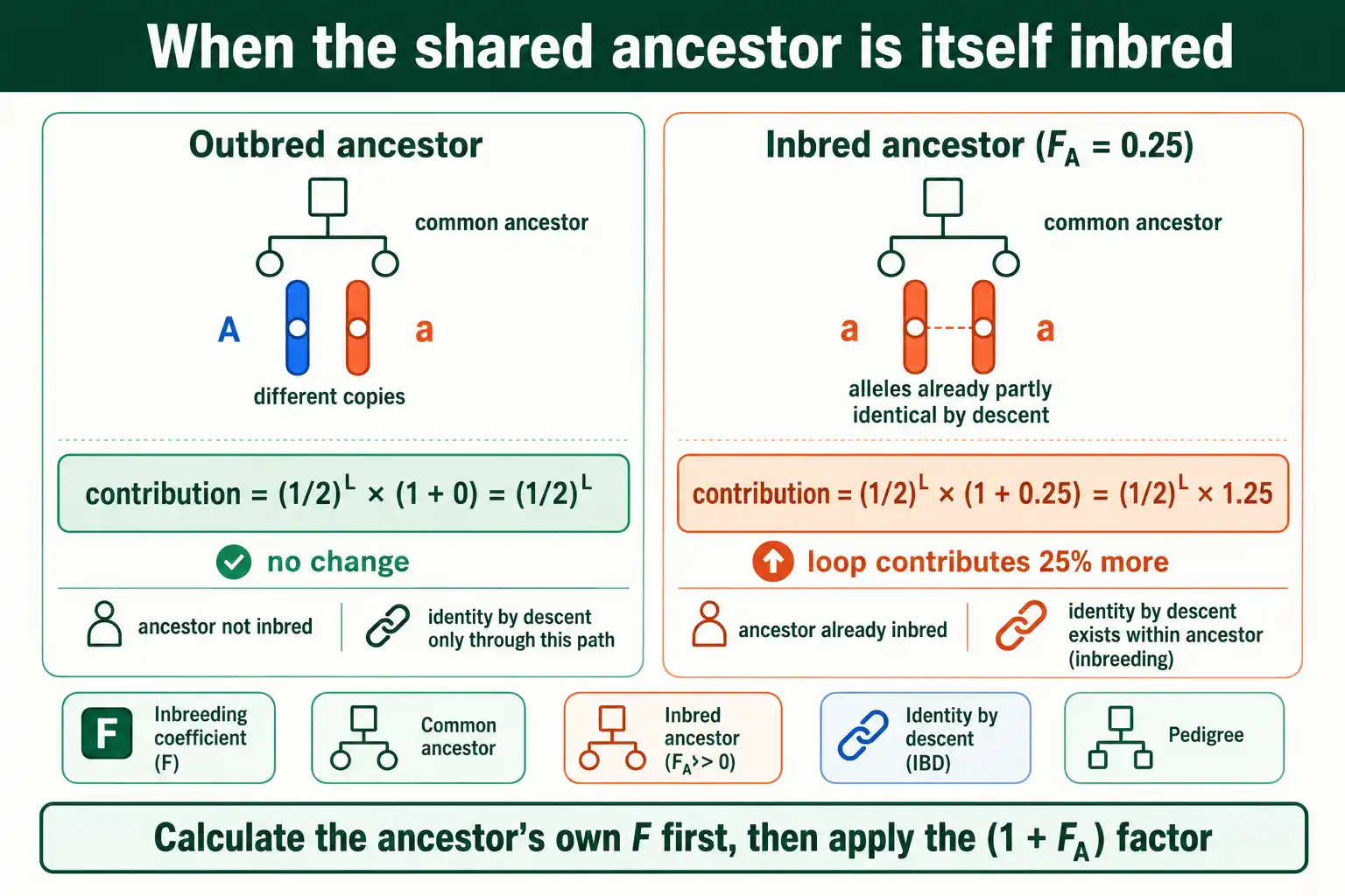
The reason is straightforward. The base method assumes the common ancestor's two alleles are not already identical by descent. If the ancestor was inbred, its two alleles already had some chance of being identical, which increases the chance it passes down identical copies. The correction multiplies that ancestor's loop contribution by (1 + F_A), where F_A is the inbreeding coefficient of the common ancestor.

So the full formula is F = Σ (1/2)^L × (1 + F_A). For an outbred common ancestor, F_A is 0, the factor becomes 1, and nothing changes, which is why the simple version works most of the time. When F_A is above 0, the loop through that ancestor contributes more.

Working it requires a preliminary step: first calculate the common ancestor's own F using the same method, then plug that value into the (1 + F_A) factor for the main calculation. For example, if a shared ancestor has an F of 0.25, its loop contributions get multiplied by 1.25, raising the final F by a quarter for those paths. The procedure nests: to find F for the individual, you sometimes first find F for an ancestor. This is also why using a truncated pedigree can mislead, because an "outbred" founder in your chart might actually have been inbred further back.

Worked Example 5: Multiple Loops

Pedigrees with several common ancestors are where people slip, because each shared ancestor adds its own loop and they all sum. A worked multi-loop case shows the bookkeeping.

Consider double first cousins. These are cousins related through both sides: their parents are two siblings married to another two siblings, so the children share all four grandparents rather than the usual two. Four common ancestors means four loops.

Each of the four loops has the same length as an ordinary first-cousin loop, contributing (1/2) to the fifth power, or 1/32. Four loops at 1/32 each sum to 4/32, which is 1/8, or 0.125. So double first cousins produce a child with an F of 0.125, exactly double the ordinary first-cousin value, and equal to half-siblings or an uncle-niece mating. The doubling comes entirely from doubling the number of shared ancestors, and so the number of loops.

The general lesson: count common ancestors carefully, because each one contributes a separate loop. Missing one undercounts F, while inventing one overcounts it. When a pedigree has many shared ancestors, listing them explicitly before tracing prevents both errors. Write down every individual who appears on both the maternal and paternal sides, then trace exactly one loop per name.

Where Path-Tracing Goes Wrong

Most calculation errors come from a handful of tracing mistakes. Naming them makes them easy to avoid.

The retracing error is the most frequent. A loop must never pass through any individual twice, including the individual whose F you are calculating. If a path doubles back through someone already in the loop, it is invalid, and counting it inflates F. Trace slowly and mark each individual as you pass through it.

The missed-ancestor error undercounts. If two of the parents' ancestors are themselves siblings or otherwise related, there may be more shared-ancestry paths than the obvious ones. Scanning only for ancestors who appear literally twice in the chart can miss loops created by relationships among the ancestors. A careful look for any relatedness among ancestors catches these.

The exponent-convention error comes from mixing formulas. Some textbooks write the contribution as (1/2)^n where n counts individuals in the loop excluding the studied individual, others as (1/2)^(n+1), and others count links rather than individuals. These all give the same answer when applied consistently, but switching between them mid-problem produces nonsense. Pick one convention, here we count the links in the loop, and hold to it.

The truncation error understates F by stopping the pedigree too early. A founder treated as outbred may have been inbred or related to another founder just beyond the chart's edge. The longer and more complete the pedigree, the more accurate the F, which is one reason genomic estimates that capture all ancestry often exceed pedigree estimates from shallow charts.

The Tabular Method for Big Pedigrees

Path-counting is ideal for human pedigrees and teaching, but it becomes unwieldy when pedigrees have hundreds of animals and tangled paths. Breeders use a different approach: the tabular method, also called the coancestry method.

Instead of tracing loops backward from an individual, the tabular method works forward through the pedigree, building a matrix of kinship between every pair of individuals generation by generation. Each individual's inbreeding coefficient equals the kinship between its two parents, read straight from the table. The method, described in Douglas Falconer and Trudy Mackay's standard text Introduction to Quantitative Genetics and systematized in early work by Lawrence Emik and Clair Terrill in a 1949 paper on calculating inbreeding coefficients, scales to enormous pedigrees because it is methodical and computer-friendly.

For regular, repeating mating systems, like continuous brother-sister mating used to create inbred laboratory strains, a third approach applies: recurrence equations. These compute each generation's F from the previous generations' values, which is far easier than tracing loops through dozens of repeated cycles. Each method suits a different situation, but all three rest on the same definition: F is the probability of identity by descent.

The recurrence approach reveals something striking about sustained inbreeding. Under continuous full-sib mating, F does not jump to 1 in one step; it climbs generation by generation, reaching about 0.25 after one generation, roughly 0.375 after two, and approaching 1 only after many generations of the same mating. This is how laboratory mouse and rat strains become almost completely homozygous, after about twenty generations of brother-sister mating, an inbred strain is treated as genetically uniform, with F effectively at 1. The slow, predictable climb is exactly what recurrence equations capture and what makes standardized inbred strains possible.

Pedigree F Versus Genomic F

Pedigree calculations give an expected F, the average identity by descent you would predict from the family tree. Modern DNA methods measure the realized F directly, and the two can differ.

The reason is chance. A pedigree predicts that the child of first cousins has an F of 0.0625, but that is an expectation across many such children. Any individual child inherits a particular random sample of chromosomes, so its actual fraction of identical-by-descent genome varies around that expected value. Some first-cousin offspring will be more inbred than 0.0625, some less.

Genomic methods estimate realized F from genetic markers in a few ways: the proportion of homozygous markers, runs of homozygosity (long stretches where both chromosomes carry identical alleles, a direct footprint of recent shared ancestry), or deviations from expected heterozygosity. These often reveal inbreeding that a short or incomplete pedigree misses, because a pedigree only captures the relatedness it records. For assessing real recessive-disease risk, the genomic estimate is increasingly the standard, while pedigree F remains valuable for planning matings before any offspring exist. The connection to homozygosity sits at the center of both, and our guide on carrier probability shows how that risk plays out for specific recessive conditions.

A Reference Table of Common Values

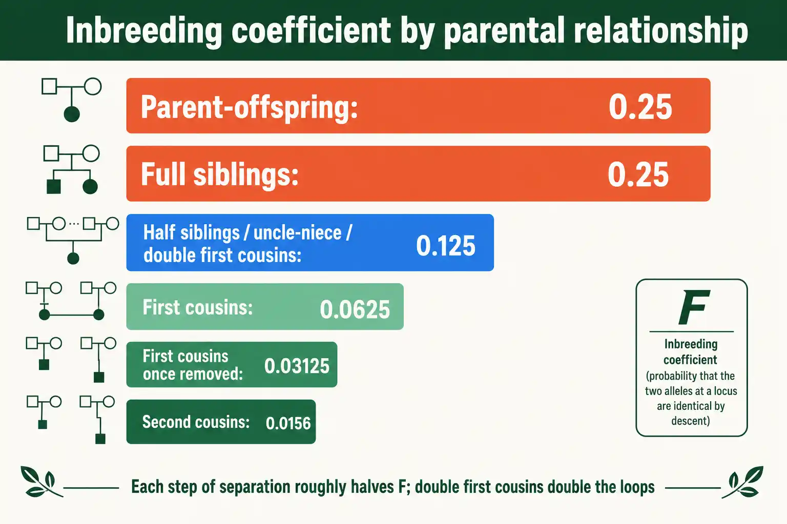
Most everyday questions involve standard relationships, and their F values are worth memorizing. The table gives the inbreeding coefficient of a child whose parents have the stated relationship.

Parents' relationship	Child's F
Parent and offspring	0.25
Full siblings	0.25
Half siblings	0.125
Uncle-niece or aunt-nephew	0.125
Double first cousins	0.125
First cousins	0.0625
First cousins once removed	0.03125
Second cousins	0.015625

A pattern runs through the table. Parent-offspring and full-sib matings both give 0.25, the highest values for non-repeated inbreeding, because the shared ancestry is immediate. Each further step of separation roughly halves F. Double first cousins reach 0.125, higher than ordinary first cousins, because they share all four grandparents instead of two, doubling the number of loops.

Checking Your Work

A few quick checks catch most errors. Run through them whenever a result looks off.

First, confirm the loop count equals the number of common ancestors. If you found three common ancestors, you should have three loops. A mismatch means a missed or doubled path.

Second, make sure no loop passes through any individual twice. Retracing a step is the single most common mistake, and it inflates F. Each loop should be a clean circuit from one parent to a common ancestor and back to the other parent.

Third, sanity-check against the reference table. If your pedigree describes first cousins but you get 0.25, something is wrong. The standard relationships are fixed reference points, and a hand calculation of a known relationship should reproduce them.

Fourth, remember the base population. F measures inbreeding relative to ancestors assumed unrelated. If your pedigree is short and those founders were actually related, your F will understate the true value. Lengthening the pedigree or estimating founder relatedness fixes this.

Frequently Asked Questions

What is the formula for the inbreeding coefficient?

F = Σ (1/2)^L × (1 + F_A), summed over every loop connecting the parents through a common ancestor. L is the number of links in the loop, and F_A is the inbreeding coefficient of that common ancestor. For outbred ancestors the (1 + F_A) term is just 1, leaving F = Σ (1/2)^L.

How do you calculate F for first cousins?

First cousins share two grandparents, giving two loops. Each loop contributes (1/2) to the fifth power, or 1/32. Summing the two loops gives 1/16, or 0.0625. That is the standard inbreeding coefficient for the child of first cousins.

Why do you sometimes add 1 to the ancestor's F?

The (1 + F_A) factor accounts for a common ancestor who was already inbred. If that ancestor's own two alleles had a chance of being identical by descent, it is more likely to pass identical copies down both lines, raising the descendant's F. You calculate the ancestor's F first, then apply the factor.

From Pedigree to Number

Calculating F comes down to a clean routine: find the common ancestors, trace each loop without repeating an individual, and sum one-half raised to each loop's length. Add the (1 + F_A) factor only when a shared ancestor was itself inbred. Wright's path method handles human pedigrees by hand, the tabular method scales to large breeding populations, and recurrence equations cover repeating systems, but all three compute the same identity-by-descent probability.

The worked cases show the logic in action: first cousins land at 0.0625, half siblings at 0.125, and an inbred ancestor pushes the figure higher. Once you can trace a loop, every standard relationship in the reference table becomes something you can derive rather than memorize. To see how the same F reads off a drawn family tree, our guide on the inbreeding coefficient from a pedigree takes it from the chart.